KPIs Configuration

Plot_KPIs creates both predefined and configurable figures. The predefined figures are:

• A map of curtailed energy for Germany and the wider region.

• A map of transmission line loading for Germany and the wider region.

• An overview plot of the energy trade.

• A summary CSV for storage capacities.

The configurable figures are defined based on config/config.kpi.yaml.

Note

The PyPSA-Eur configuration files follow a pyramid-like structure, where the parameters in the highest configuration file add to and override those in the configuration file below it. The order is as follows:

1. scenarios.form.yaml

2. config.form.yaml

3. config.default.yaml

4. config.kpi.yaml (this section)

Thus, for example changes specified in scenario.form.yaml will add to and override configurations in config.form.yaml and so on.

Key components of each configuration:

1. extract: Defines the network statistics for the figures (e.g., system cost, generation, storage, emissions).

2. include and/or exclude: Specifies the regions or entities to include or exclude in the calculation (e.g., “DE” for Germany, “EU” for the European Union).

3. carrier_filter: Specifies the energy carriers or technologies (e.g., power, electricity, storage, heat) relevant to the figure.

4. group_carrier: Specifies the names used for each carrier. Same names are aggregated.

5. plot: Determines the type of plot or visualization to be used (e.g., “detail” for detailed data, “overview” for broader data representation).

6. figsize: Determines the figsize of the plots. If not defined, the default size are chosen.

7. plot_kw: Additional keyword arguments for the plot (e.g., title, labels, and axis).

Note

The head of the config/config.kpi.yaml file includes two options that will affect all plots:

• enable_latex: Saves the plot in LaTeX format.

• include_csvs: Saves a CSV file for each plot generated.

Components

extract

• system cost: Extract data from csvs/nodal_costs.csv.

• capacity: Extract data from csvs/nodal_capacities.csv.

• capacity stats: Extract capacity data from n.statistics. See notes for more detail.

• generation: Extract power generation data from n.statistics.energy_balance.

• curtailment: Extract power generation data from n.statistics.curtailment.

• emission: Extract emissions data based on emission links to the atmosphere.

• energy balance: Extract energy balance data from n.statistics.energy_balance.

• SOC: Extract state of charge from the storage_units component.

Note

capacity stats is a special option because it has two extra components:

stats: Extract capacity data from these three options:

• install: Extract capacity data from n.statistics.installed_capacity

• optimal: (Default) Extract capacity data from n.statistics.optimal_capacity

• expand: The difference between optimal minus install.

storage: If set to true, only storage capacities of the component store and storage_units are taken into account.

carrier_filter

a. for system cost, capacity, capacity stats, generation, and emission:

• electricity: Filter carrier with AC bus carrier.

• electricity+: Filter carrier with AC bus carrier and also include water tanks and EV batteries.

• storage: Filter carrier with all storage-related technologies (storage_units, links, and stores).

• storage-cap: Filter carrier with all storage capacity-related technologies (storage_units and links).

• storage-energy: Filter carrier with all storage energy-related technologies (storage_units and stores).

• power: Filter carrier with power generation technologies.

Note

storage, storage-cap, storage-energy, power is based on a list in config/config.kpi.yaml. You can create your own filtering scheme by adding a list in kpi: filter_scheme

    power: [
      "solar rooftop","Solar","solar-hsat","Onshore Wind","Offshore Wind (DC)",
      "Offshore Wind (AC)","Offshore Wind (Floating)","Run of River","Reservoir & Dam",
      "Open-Cycle Gas","Combined-Cycle Gas","nuclear","oil","lignite","coal"
      ]

b. for energy balance:

• electricity: Filter carrier with AC bus carrier.

• electricity+: Filter carrier with AC bus carrier and also include solar rooftops, BEV chargers, and Vehicle-to-Gas.

• low voltage: Filter carrier with low voltage bus carrier.

• storage: Filter carrier with all storage capacity-related technologies.

• heat: Filter carrier with heat bus carrier.

• hydrogen: Filter carrier with hydrogen bus carrier.

c. for SOC, this can be defined individually or in arrays of storage_units carriers.

group_carrier

• pretty: The first letter is capitalized, abbreviations are spelled out, and similar names are combined.

• sector: Aggregate all technologies into either the power sector, heating, transport sector, primary fuel, or CCUS.

Leaving this option empty will lead to the carriers using nice_names.

plot

for system cost, capacity, capacity stats, generation, and emission:

• detail: A single bar plot is created with all the values annotated.

• overview: Multiple bar plots are created.

The plot for energy balance and SOC is always in a time-series format.

figsize

• For detail plots: the default figsize is (6,8)

• For overview, energy balance and SOC plots: the default figsize is (12,9)

plot_kw

• For system cost, capacity, capacity stats, generation, and emission, see matplotlib.pyplot.bar documentation.

• For energy balance and SOC, see pandas.DataFrame.plot documentation.

Examples

Detail Plots

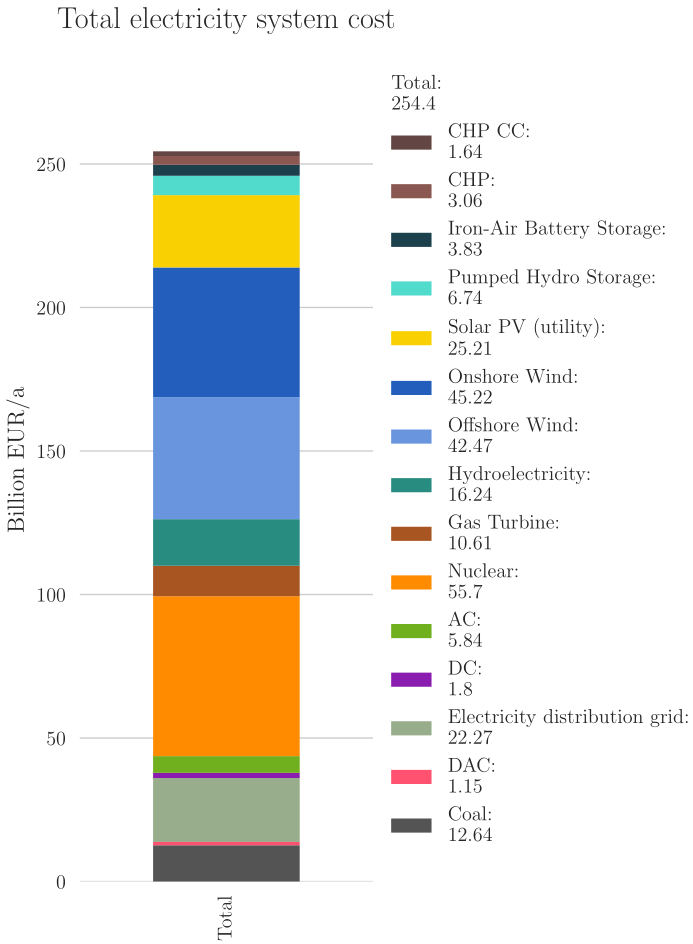
    All_electricity_system_cost:
      extract: system cost
      carrier_filter: electricity
      group_carrier: pretty
      plot: detail
      plot_kw:
        title: Total electricity system cost
        #ylim: [0,350]
        ylabel: Billion EUR/a

Explaination:

• A detail plot is one that displays the value of each carrier on the right side of a single bar plot.

• In this example, the value represented is the system cost.

• This plot includes only the carriers related to electricity.

• The carrier names are based on the pretty_names defined in plot_KPIs.py.

• The title of the plot is Total electricity system cost, with the unit in Billion EUR/a.

• The file is saved as {postnetwork}-All_electricity_system_cost_{planning_horizon}.pdf.

The results are the figure below:

Overview Plots

    country_storage_energy_capacity:
      extract: capacity stats
      storage: true
      exclude: ["EU"]
      carrier_filter: storage-energy
      group_carrier: pretty
      plot: overview
      plot_kw:
        title: Country storage energy capacity
        #ylim: [0,5000]
        ylabel: GWh

Explaination:

• An overview plot displays the value of each carrier for all countries that are included, excluding those that are not relevant.

• ["EU"] refers to buses that do not belong to any specific country. In this context, they are excluded from the plots as they are not relevant.

• In this example, the value represented is capacity stats.

  • Since stats is not specified, the default optimal is chosen, and the data is extracted from n.statistics.optimal_capacity.

  • As store is set to true, the data for storage capacities is extracted.

• This plot includes only the carriers listed in storage-cap.

• The carrier names are based on the pretty_names defined in plot_KPIs.py.

• The title of the plot is Country storage power capacity with the unit in GWe.

• The file is saved as {postnetwork}-country_storage_power_capacity_{planning_horizon}.pdf.

The results are the figure below:

Time Series Plots

    DE_electricity_summer_energy_balance:
      extract: energy balance
      include: ["DE"]
      carrier_filter: electricity+
      group_carrier: pretty
      plot_kw:
        title: Germany summer high and low voltage energy balance
        xlim: ['2013-08-01', '2013-09-01']
        #ylim: [-50,200]
        ylabel: GW

Explaination:

• The value represented in this plot is the energy balance.

• Energy balance means the resulting plot will be a time series (no need for a plot definition).

• This plot includes only the carriers related to electricity+ which covers the high voltage carrier, as well as some low voltage generators such as PV (rooftop) and storages such as Battery Electric Vehicles.

• The carrier names are based on the pretty_names defined in plot_KPIs.py.

• The title of the plot is Germany summer high and low voltage energy balance, with the unit in GW.

• The time series plot is limited to the snapshot dates between 2013-08-01 and 2013-09-01.

• The file is saved as {postnetwork}-DE_electricity_summer_energy_balance_{planning_horizon}.pdf.

The results are the figure below: