Workshop 1: Introduction to PyPSA & TYNDP reference grids

PyPSA stands for Python for Power System Analysis.

PyPSA is an open source Python package for simulating and optimising modern energy systems that include features such as

• conventional generators with unit commitment (ramp-up, ramp-down, start-up, shut-down),

• time-varying wind and solar generation,

• energy storage with efficiency losses and inflow/spillage for hydroelectricity

• coupling to other energy sectors (electricity, transport, heat, industry),

• conversion between energy carriers (e.g. electricity to hydrogen),

• transmission networks (AC, DC, other fuels)

PyPSA can be used for a variety of problem types (e.g. electricity market modelling, long-term investment planning, transmission network expansion planning), and is designed to scale well with large networks and long time series.

Compared to building power system by hand in linopy, PyPSA does the following things for you:

• manage data inputs

• build optimisation problem

• communicate with the solver

• retrieve and process optimisation results

• manage data outputs

Dependencies

• pandas for storing data about network components and time series

• numpy and scipy for linear algebra and sparse matrix calculations

• matplotlib and cartopy for plotting on a map

• networkx for network calculations

• linopy for handling optimisation problems

Note

Documentation for this package is available at https://pypsa.readthedocs.io.

Basic Structure

Component	Description
Network	Container for all components.
Bus	Node where components attach.
Carrier	Energy carrier or technology (e.g. electricity, hydrogen, gas, coal, oil, biomass, on-/offshore wind, solar). Can track properties such as specific carbon dioxide emissions or nice names and colors for plots.
Load	Energy consumer (e.g. electricity demand).
Generator	Generator (e.g. power plant, wind turbine, PV panel).
Link	Links connect two buses with controllable energy flow, direction-control and losses. They can be used to model: HVDC links HVAC lines (neglecting KVL, only net transfer capacities (NTCs)) conversion between carriers (e.g. electricity to hydrogen in electrolysis)
GlobalConstraint	Constraints affecting many components at once, such as emission limits.
Not covered in this workshop
Line	Power distribution and transmission lines (overhead and cables).
LineType	Standard line types.
Transformer	2-winding transformer.
TransformerType	Standard types of 2-winding transformer.
ShuntImpedance	Shunt.
StorageUnit	Storage with fixed nominal energy-to-power ratio.
Store	Storage with separately extendable energy capacity.

Note

Links in the table lead to documentation for each component.

Warning

Per unit values of voltage and impedance are used internally for network calculations. It is assumed internally that the base power is 1 MW.

From structured data to optimisation

The design principle of PyPSA is that basically each component is associated with a set of variables and constraints that will be added to the optimisation model based on the input data stored for the components.

For an hourly electricity market simulation, PyPSA will solve an optimisation problem that looks like this

(1)\[\begin{equation} \min_{g_{i,s,t}; f_{\ell,t}; g_{i,r,t,\text{charge}}; g_{i,r,t,\text{discharge}}; e_{i,r,t}} \sum_s o_{s} g_{i,s,t} \end{equation}\]

such that

(2)\[\begin{align} 0 & \leq g_{i,s,t} \leq \hat{g}_{i,s,t} G_{i,s} & \text{generation limits : generator} \\ -F_\ell &\leq f_{\ell,t} \leq F_\ell & \text{transmission limits : line} \\ d_{i,t} &= \sum_s g_{i,s,t} + \sum_r g_{i,r,t,\text{discharge}} - \sum_r g_{i,r,t,\text{charge}} - \sum_\ell K_{i\ell} f_{\ell,t} & \text{KCL : bus} \\ 0 &=\sum_\ell C_{\ell c} x_\ell f_{\ell,t} & \text{KVL : cycles} \\ 0 & \leq g_{i,r,t,\text{discharge}} \leq G_{i,r,\text{discharge}}& \text{discharge limits : storage unit} \\ 0 & \leq g_{i,r,t,\text{charge}} \leq G_{i,r,\text{charge}} & \text{charge limits : storage unit} \\ 0 & \leq e_{i,r,t} \leq E_{i,r} & \text{energy limits : storage unit} \\ e_{i,r,t} &= \eta^0_{i,r,t} e_{i,r,t-1} + \eta^1_{i,r,t}g_{i,r,t,\text{charge}} - \frac{1}{\eta^2_{i,r,t}} g_{i,r,t,\text{discharge}} & \text{consistency : storage unit} \\ e_{i,r,0} & = e_{i,r,|T|-1} & \text{cyclicity : storage unit} \end{align}\]

Decision variables:

• \(g_{i,s,t}\) is the generator dispatch at bus \(i\), technology \(s\), time step \(t\),

• \(f_{\ell,t}\) is the power flow in line \(\ell\),

• \(g_{i,r,t,\text{dis-/charge}}\) denotes the charge and discharge of storage unit \(r\) at bus \(i\) and time step \(t\),

• \(e_{i,r,t}\) is the state of charge of storage \(r\) at bus \(i\) and time step \(t\).

Parameters:

• \(o_{i,s}\) is the marginal generation cost of technology \(s\) at bus \(i\),

• \(x_\ell\) is the reactance of transmission line \(\ell\),

• \(K_{i\ell}\) is the incidence matrix,

• \(C_{\ell c}\) is the cycle matrix,

• \(G_{i,s}\) is the nominal capacity of the generator of technology \(s\) at bus \(i\),

• \(F_{\ell}\) is the rating of the transmission line \(\ell\),

• \(E_{i,r}\) is the energy capacity of storage \(r\) at bus \(i\),

• \(\eta^{0/1/2}_{i,r,t}\) denote the standing (0), charging (1), and discharging (2) efficiencies.

Note

For a full reference to the optimisation problem description, see https://pypsa.readthedocs.io/en/latest/optimal_power_flow.html

Introduction to pypsa: a minimal dispatch problem

Copyright (c) 2025, Iegor Riepin

Note

If you have not yet set up Python on your computer, you can execute this tutorial in your browser via Google Colab. Click on the rocket in the top right corner and launch “Colab”. If that doesn’t work download the .ipynb file and import it in Google Colab.

Then install the following packages by executing the following command in a Jupyter cell at the top of the notebook.

!pip install pypsa atlite pandas geopandas xarray matplotlib hvplot geoviews plotly highspy holoviews folium mapclassify

# To run this notebook in Google Colab, uncomment the following line:
# !pip install pypsa atlite pandas geopandas xarray matplotlib hvplot geoviews plotly highspy holoviews folium mapclassify

# By convention, PyPSA is imported without an alias:
import pypsa

# Other dependencies
import pandas as pd
import geopandas as gpd
import matplotlib.pyplot as plt
import holoviews as hv
import hvplot.pandas
import cartopy.crs as ccrs
import folium
import mapclassify
from pypsa.plot.maps.static import (
    add_legend_circles,
    add_legend_patches,
    add_legend_lines,
)
from pathlib import Path

plt.style.use("bmh")

Minimal electricity market problem

generator 1: “gas” – marginal cost 70 EUR/MWh – capacity 50 MW

generator 2: “nuclear” – marginal cost 10 EUR/MWh – capacity 100 MW

load: “Consumer” – demand 120 MW

single time step (“now”)

single node (“Springfield”)

Building a basic network

# First, we create a network object which serves as the container for all components
n1 = pypsa.Network(name="Demo")

n1

Empty PyPSA Network 'Demo'
--------------------
Components: none
Snapshots: 1

The second component we need are buses. Buses are the fundamental nodes of the network, to which all other components like loads, generators and transmission lines attach. They enforce energy conservation for all elements feeding in and out of it (i.e. Kirchhoff’s Current Law).

Components can be added to the network n using the n.add() function. It takes the component name as a first argument, the name of the component as a second argument and possibly further parameters as keyword arguments. Let’s use this function, to add buses for each country to our network:

n1.add("Carrier", "AC")
n1.add("Bus", "Springfield", v_nom=380, carrier="AC")

Index(['Springfield'], dtype='object')

For each class of components, the data describing the components is stored in a pandas.DataFrame. For example, all static data for buses is stored in n.buses

n1.buses

	v_nom	type	x	y	carrier	unit	location	v_mag_pu_set	v_mag_pu_min	v_mag_pu_max	control	generator	sub_network
Bus
Springfield	380.0		0.0	0.0	AC			1.0	0.0	inf	PQ

You see there are many more attributes than we specified while adding the buses; many of them are filled with default parameters which were added. You can look up the field description, defaults and status (required input, optional input, output) for buses here https://pypsa.readthedocs.io/en/latest/components.html#bus, and analogous for all other components.

You can also explore attributes yourself.

n1.component_attrs["Bus"]
# n1.component_attrs["Generator"]
# n1.component_attrs["Link"]
# n1.component_attrs["Load"]

	type	unit	default	description	status	static	varying	typ	dtype
attribute
name	string	NaN		Unique name	Input (required)	True	False	<class 'str'>	object
v_nom	float	kV	1.0	Nominal voltage	Input (optional)	True	False	<class 'float'>	float64
type	string	NaN		Placeholder for bus type. Not yet implemented.	Input (optional)	True	False	<class 'str'>	object
x	float	NaN	0.0	Position (e.g. longitude); the Spatial Referen...	Input (optional)	True	False	<class 'float'>	float64
y	float	NaN	0.0	Position (e.g. latitude); the Spatial Referenc...	Input (optional)	True	False	<class 'float'>	float64
carrier	string	NaN	AC	Energy carrier: can be "AC" or "DC" for electr...	Input (optional)	True	False	<class 'str'>	object
unit	string	NaN		Unit of the bus’ carrier if the implicitly ass...	Input (optional)	True	False	<class 'str'>	object
location	string	NaN		Location of the bus. Does not influence the op...	Input (optional)	True	False	<class 'str'>	object
v_mag_pu_set	static or series	per unit	1.0	Voltage magnitude set point, per unit of v_nom.	Input (optional)	True	True	<class 'float'>	float64
v_mag_pu_min	float	per unit	0.0	Minimum desired voltage, per unit of v_nom. Th...	Input (optional)	True	False	<class 'float'>	float64
v_mag_pu_max	float	per unit	inf	Maximum desired voltage, per unit of v_nom. T...	Input (optional)	True	False	<class 'float'>	float64
control	string	NaN	PQ	P,Q,V control strategy for PF, must be "PQ", "...	Output	True	False	<class 'str'>	object
generator	string	NaN		Name of slack generator attached to slack bus.	Output	True	False	<class 'str'>	object
sub_network	string	NaN		Name of connected sub-network to which bus bel...	Output	True	False	<class 'str'>	object
p	series	MW	0.0	active power at bus (positive if net generatio...	Output	False	True	<class 'float'>	float64
q	series	MVar	0.0	reactive power (positive if net generation at ...	Output	False	True	<class 'float'>	float64
v_mag_pu	series	per unit	1.0	Voltage magnitude, per unit of v_nom	Output	False	True	<class 'float'>	float64
v_ang	series	radians	0.0	Voltage angle	Output	False	True	<class 'float'>	float64
marginal_price	series	currency/MWh	0.0	Locational marginal price from LOPF from power...	Output	False	True	<class 'float'>	float64

The n.add() function lets you add any component to the network object n:

n1.add(
    "Generator",
    "gas",
    carrier="AC",
    bus="Springfield",
    p_nom_extendable=False,
    marginal_cost=70,  # €/MWh
    p_nom=50,  # MW
)
n1.add(
    "Generator",
    "nuclear",
    carrier="AC",
    bus="Springfield",
    p_nom_extendable=False,
    marginal_cost=10,  # €/MWh
    p_nom=100,  # MW
)

Index(['nuclear'], dtype='object')

The method n.add() also allows you to add multiple components at once. For instance, multiple carriers for the fuels with information on specific carbon dioxide emissions, a nice name, and colors for plotting. For this, the function takes the component name as the first argument and then a list of component names and then optional arguments for the parameters. Here, scalar values, lists, dictionary or pandas.Series are allowed. The latter two needs keys or indices with the component names.

As a result, the n.generators DataFrame looks like this:

n1.generators

	bus	control	type	p_nom	p_nom_mod	p_nom_extendable	p_nom_min	p_nom_max	p_min_pu	p_max_pu	...	min_up_time	min_down_time	up_time_before	down_time_before	ramp_limit_up	ramp_limit_down	ramp_limit_start_up	ramp_limit_shut_down	weight	p_nom_opt
Generator
gas	Springfield	PQ		50.0	0.0	False	0.0	inf	0.0	1.0	...	0	0	1	0	NaN	NaN	1.0	1.0	1.0	0.0
nuclear	Springfield	PQ		100.0	0.0	False	0.0	inf	0.0	1.0	...	0	0	1	0	NaN	NaN	1.0	1.0	1.0	0.0

2 rows × 37 columns

Next, we’re going to add the electricity demand.

A positive value for p_set means consumption of power from the bus.

n1.add(
    "Load",
    "Small town",
    carrier="AC",
    bus="Springfield",
    p_set=120,  # MW
)

Index(['Small town'], dtype='object')

n1.loads

	bus	carrier	type	p_set	q_set	sign	active
Load
Small town	Springfield	AC		120.0	0.0	-1.0	True

Optimisation

The design principle of PyPSA is that basically each component is associated with a set of variables and constraints that will be added to the optimisation model based on the input data stored for the components.

For this dispatch problem, PyPSA will solve an optimisation problem that looks like this

(3)\[\begin{equation} \min_{g_{s,t};} \sum_{t,s} o_{s} g_{s,t} \end{equation}\]

such that

(4)\[\begin{align} 0 & \leq g_{s,t} \leq G_{s} & \text{generation limits : generator} \\ D_t &= \sum_s g_{s,t} & \text{market clearing : bus} \\ \end{align}\]

Decision variables:

• \(g_{s,t}\) is the generator dispatch of technology \(s\) at time \(t\)

Parameters:

• \(o_{s}\) is the marginal generation cost of technology \(s\)

• \(G_{s}\) is the nominal capacity of technology \(s\)

• \(D_t\) is the power demand in Springfiled at time \(t\)

With all input data transferred into the PyPSA’s data structure (network), we can now build and run the resulting optimisation problem. In PyPSA, building, solving and retrieving results from the optimisation model is contained in a single function call n.optimize(). This function optimizes dispatch and investment decisions for least cost adhering to the constraints defined in the network.

The n.optimize() function can take a variety of arguments. The most relevant for the moment is the choice of the solver (e.g. “highs” and “gurobi”). They need to be installed on your computer, to use them here!

n1.optimize(solver_name="highs")

INFO:linopy.model: Solve problem using Highs solver

INFO:linopy.io: Writing time: 0.01s

INFO:linopy.constants: Optimization successful: 
Status: ok
Termination condition: optimal
Solution: 2 primals, 5 duals
Objective: 2.40e+03
Solver model: available
Solver message: optimal

INFO:pypsa.optimization.optimize:The shadow-prices of the constraints Generator-fix-p-lower, Generator-fix-p-upper were not assigned to the network.

Running HiGHS 1.10.0 (git hash: fd86653): Copyright (c) 2025 HiGHS under MIT licence terms
LP   linopy-problem-4tgp1exh has 5 rows; 2 cols; 6 nonzeros
Coefficient ranges:
  Matrix [1e+00, 1e+00]
  Cost   [1e+01, 7e+01]
  Bound  [0e+00, 0e+00]
  RHS    [5e+01, 1e+02]
Presolving model
0 rows, 0 cols, 0 nonzeros  0s
0 rows, 0 cols, 0 nonzeros  0s
Presolve : Reductions: rows 0(-5); columns 0(-2); elements 0(-6) - Reduced to empty
Solving the original LP from the solution after postsolve
Model name          : linopy-problem-4tgp1exh
Model status        : Optimal
Objective value     :  2.4000000000e+03
Relative P-D gap    :  0.0000000000e+00
HiGHS run time      :          0.00
Writing the solution to /tmp/linopy-solve-mlupkymc.sol

('ok', 'optimal')

Let’s have a look at the results. The network object n contains now the objective value and the results for the decision variables.

n1.objective

2400.0

Since the power flow and dispatch are generally time-varying quantities, these are stored in a different locations than e.g. n.generators. They are stored in n.generators_t. Thus, to find out the dispatch of the generators, run

n1.generators_t.p

Generator	gas	nuclear
snapshot
now	20.0	100.0

n1.buses_t.marginal_price

Bus	Springfield
snapshot
now	70.0

Explore pypsa model

n1.model

Linopy LP model
===============

Variables:
----------
 * Generator-p (snapshot, Generator)

Constraints:
------------
 * Generator-fix-p-lower (snapshot, Generator-fix)
 * Generator-fix-p-upper (snapshot, Generator-fix)
 * Bus-nodal_balance (Bus, snapshot)

Status:
-------
ok

n1.model.constraints

linopy.model.Constraints
------------------------
 * Generator-fix-p-lower (snapshot, Generator-fix)
 * Generator-fix-p-upper (snapshot, Generator-fix)
 * Bus-nodal_balance (Bus, snapshot)

n1.model.constraints["Generator-fix-p-upper"]

Constraint `Generator-fix-p-upper` [snapshot: 1, Generator-fix: 2]:
-------------------------------------------------------------------
[now, gas]: +1 Generator-p[now, gas]         ≤ 50.0
[now, nuclear]: +1 Generator-p[now, nuclear] ≤ 100.0

n1.model.constraints["Bus-nodal_balance"]

Constraint `Bus-nodal_balance` [Bus: 1, snapshot: 1]:
-----------------------------------------------------
[Springfield, now]: +1 Generator-p[now, gas] + 1 Generator-p[now, nuclear] = 120.0

n1.model.objective

Objective:
----------
LinearExpression: +70 Generator-p[now, gas] + 10 Generator-p[now, nuclear]
Sense: min
Value: 2400.0

Exercise 1: Add another town to the model

The new town Shelbyville consists of:

• one coal power plant with a capacity of 100 MW and marginal cost of 50 €/MWh

• a transmission line with net transfer capacity of 10 MW

• a Load of 70 MW

!Hint: you can use the link component to add NTC representations of transmission lines like this:

n.add(
    "Link",
    Transmission Line, 
    bus0="TownA", 
    bus1="TownB", 
    p_nom=..., 
    carrier="AC", 
    p_min_pu=-1  # For bidirectional links
)

# Your solution

Building the reference grids

The minimal PyPSA example illustrates how time-consuming it can be to compose a network by hand. To simplify the work, PyPSA-Eur provides a set of scripts that does this for you. It collects and processes open data, composes a network, writes the constraints, solves the operation and capacity expansion problem, collects the result and produces basic summary outputs for analysis.

The current open-tyndp project aims to adapt PyPSA-Eur to the specific needs of the TYNDP process. All the code is openly available in the project repository: open-tyndp. Currently, the workflow implements the reference grid data for both the electricity and hydrogen networks and solves the network with the default PyPSA-Eur demand.

As any open-source repository, you can get the code, contribute using pull-requests, reports issues and submit feature requests.

Load example data

For this workshop, we have prepared networks that can be explored immediately:

• pre-network: The network prepared by the workflow before solving it.

• post-network: The solved network.

As this workshop focuses on the reference grid, we will also explore the bidding zones data we have created.

from urllib.request import urlretrieve

urls = {
    "pre-network.nc": "https://drive.usercontent.google.com/download?id=17b7YZGXKczY2K5sRPUDJkD5AVwgbOgAh&export=download",
    "post-network.nc": "https://drive.usercontent.google.com/download?id=1qIN0tlZBACPtKCBxHUpBAecBqYsy-sTV&export=download&confirm=t&uuid=cf9cb5cf-de33-4ef4-9f49-5f01f2d571b1",
    "bidding_zones.geojson": "https://drive.usercontent.google.com/download?id=12xpT5TQrvlkEY3maIhXH_2sliJ3K7T0r&export=download",
}
for name, url in urls.items():
    print(f"Retrieving {name} from Google Drive")
    urlretrieve(url, name)
print("Done")

Retrieving pre-network.nc from Google Drive

Retrieving post-network.nc from Google Drive

Retrieving bidding_zones.geojson from Google Drive

Done

First, let’s load a pre-composed PyPSA Network:

n2 = pypsa.Network("pre-network.nc")

INFO:pypsa.io:Imported network pre-network.nc has buses, carriers, generators, global_constraints, links, loads, shapes, storage_units, stores

And let’s get a general overview of the components in it:

n2

PyPSA Network 'PyPSA-Eur (tyndp-raw)'
-------------------------------------
Components:
 - Bus: 680
 - Carrier: 101
 - Generator: 661
 - GlobalConstraint: 2
 - Link: 2338
 - Load: 338
 - Shape: 62
 - StorageUnit: 69
 - Store: 350
Snapshots: 1460

We have buses which represent the different nodes in the model where components attach.

n2.buses.head()

	v_nom	type	x	y	carrier	unit	location	v_mag_pu_set	v_mag_pu_min	v_mag_pu_max	control	generator	sub_network	substation_lv	substation_off	country
Bus
AL00	380.0		20.036884	41.117588	AC	MWh_el	AL00	1.0	0.0	inf	PQ			1.0	1.0	AL
AT00	380.0		14.822183	47.668898	AC	MWh_el	AT00	1.0	0.0	inf	PQ			1.0	1.0	AT
BA00	380.0		17.867837	43.982016	AC	MWh_el	BA00	1.0	0.0	inf	PQ			1.0	1.0	BA
BE00	380.0		4.967931	50.470635	AC	MWh_el	BE00	1.0	0.0	inf	PQ			1.0	1.0	BE
BG00	380.0		25.323948	42.668760	AC	MWh_el	BG00	1.0	0.0	inf	PQ			1.0	1.0	BG

And let’s look at electric buses for a specific country.

n2.buses.query("country=='IT' and carrier=='AC'")

	v_nom	type	x	y	carrier	unit	location	v_mag_pu_set	v_mag_pu_min	v_mag_pu_max	control	generator	sub_network	substation_lv	substation_off	country
Bus
ITCA	380.0		16.634892	38.985885	AC	MWh_el	ITCA	1.0	0.0	inf	PQ			1.0	1.0	IT
ITCN	380.0		11.238605	43.418039	AC	MWh_el	ITCN	1.0	0.0	inf	PQ			1.0	1.0	IT
ITCS	380.0		13.162117	41.846461	AC	MWh_el	ITCS	1.0	0.0	inf	PQ			1.0	1.0	IT
ITN1	380.0		9.703872	45.440276	AC	MWh_el	ITN1	1.0	0.0	inf	PQ			1.0	1.0	IT
ITS1	380.0		16.501565	40.927422	AC	MWh_el	ITS1	1.0	0.0	inf	PQ			1.0	1.0	IT
ITSA	380.0		9.097371	40.067626	AC	MWh_el	ITSA	1.0	0.0	inf	PQ			1.0	1.0	IT
ITSI	380.0		13.863833	37.546811	AC	MWh_el	ITSI	1.0	0.0	inf	PQ			1.0	1.0	IT
ITVI	380.0		13.863833	37.546811	AC	MWh_el	ITVI	1.0	0.0	inf	PQ			0.0	0.0	IT
IT H2 Z2 DRES	380.0		16.634892	38.985885	AC	MWh_el	IT H2 Z2	1.0	0.0	inf	PQ			1.0	1.0	IT

Generators which represent generating units (e.g. wind turbine, PV panel):

n2.generators.head()

	bus	control	type	p_nom	p_nom_mod	p_nom_extendable	p_nom_min	p_nom_max	p_min_pu	p_max_pu	...	up_time_before	down_time_before	ramp_limit_up	ramp_limit_down	ramp_limit_start_up	ramp_limit_shut_down	weight	p_nom_opt	location	unit
Generator
AL00 offwind-ac	AL00	PQ		0.000000	0.0	True	0.000000	3160.441247	0.0	1.0	...	1	0	NaN	NaN	1.0	1.0	1.0	0.0
BA00 offwind-ac	BA00	PQ		0.000000	0.0	True	0.000000	16.871211	0.0	1.0	...	1	0	NaN	NaN	1.0	1.0	1.0	0.0
BE00 offwind-ac	BE00	PQ		1053.971009	0.0	True	1053.971009	1053.971009	0.0	1.0	...	1	0	NaN	NaN	1.0	1.0	1.0	0.0
BG00 offwind-ac	BG00	PQ		0.000000	0.0	True	0.000000	1598.925797	0.0	1.0	...	1	0	NaN	NaN	1.0	1.0	1.0	0.0
CY00 offwind-ac	CY00	PQ		0.000000	0.0	True	0.000000	2057.040496	0.0	1.0	...	1	0	NaN	NaN	1.0	1.0	1.0	0.0

5 rows × 39 columns

Links connect two buses with controllable energy flow, direction-control and losses. They can be used to model:

• HVAC lines (neglecting KVL, only net transfer capacities (NTCs))
• HVDC links
• conversion between carriers (e.g. electricity to hydrogen in electrolysis)

PyPSA-Eur uses DC as the conventional carrier for electrical transmission lines modelled as Link. AC is used as the conventional carrier for electrical transmission Line.

n2.links.head()

	bus0	bus1	type	carrier	efficiency	active	build_year	lifetime	p_nom	p_nom_mod	...	voltage	dc	energy to power ratio	reversed	underwater_fraction	tags	bidirectional	location	length_original	geometry
Link
AL00-GR00-DC	AL00	GR00		DC	1.0	True	0	inf	600.0	0.0	...	380.0	1.0	NaN	False	0.0	AL00 -> GR00	NaN		219.635111	LINESTRING (20.036883988642362 41.117587702511...
AL00-ME00-DC	AL00	ME00		DC	1.0	True	0	inf	400.0	0.0	...	380.0	1.0	NaN	False	0.0	AL00 -> ME00	NaN		189.342890	LINESTRING (20.036883988642362 41.117587702511...
AL00-MK00-DC	AL00	MK00		DC	1.0	True	0	inf	500.0	0.0	...	380.0	1.0	NaN	False	0.0	AL00 -> MK00	NaN		153.308707	LINESTRING (20.036883988642362 41.117587702511...
AL00-RS00-DC	AL00	RS00		DC	1.0	True	0	inf	250.0	0.0	...	380.0	1.0	NaN	False	0.0	AL00 -> RS00	NaN		351.420535	LINESTRING (20.036883988642362 41.117587702511...
AT00-CH00-DC	AT00	CH00		DC	1.0	True	0	inf	1200.0	0.0	...	380.0	1.0	NaN	False	0.0	AT00 -> CH00	NaN		502.028400	LINESTRING (14.822183225330722 47.668898155000...

5 rows × 52 columns

You can filter a country.

n2.links.query("Link.str.contains('DE')").head()

	bus0	bus1	type	carrier	efficiency	active	build_year	lifetime	p_nom	p_nom_mod	...	voltage	dc	energy to power ratio	reversed	underwater_fraction	tags	bidirectional	location	length_original	geometry
Link
AT00-DE00-DC	AT00	DE00		DC	1.0	True	0	inf	7500.0	0.0	...	380.0	1.0	NaN	False	0.0	AT00 -> DE00	NaN		512.754700	LINESTRING (14.822183225330722 47.668898155000...
BE00-DE00-DC	BE00	DE00		DC	1.0	True	0	inf	1000.0	0.0	...	380.0	1.0	NaN	False	0.0	BE00 -> DE00	NaN		369.599774	LINESTRING (4.96793113501169 50.47063494467691...
CH00-DE00-DC	CH00	DE00		DC	1.0	True	0	inf	4200.0	0.0	...	380.0	1.0	NaN	False	0.0	CH00 -> DE00	NaN		503.448277	LINESTRING (8.343016848147014 46.7336228266206...
CZ00-DE00-DC	CZ00	DE00		DC	1.0	True	0	inf	2600.0	0.0	...	380.0	1.0	NaN	False	0.0	CZ00 -> DE00	NaN		422.050833	LINESTRING (15.66368315845627 49.7526624846696...
DE00-AT00-DC	DE00	AT00		DC	1.0	True	0	inf	7500.0	0.0	...	380.0	1.0	NaN	False	0.0	DE00 -> AT00	NaN		512.754700	LINESTRING (10.11340015140031 51.1099148631177...

5 rows × 52 columns

The workflow also attaches Load to the network. As the load is a time sensitive information, the data is stored in n.loads_t. The provided network uses the default PyPSA-Eur loads.

n2.loads_t.p_set.head()

Load	AL00	AL00 rural heat	AL00 urban central heat	AL00 urban decentral heat	AT00	AT00 rural heat	AT00 urban central heat	AT00 urban decentral heat	BA00	BA00 rural heat	...	SE04 urban central heat	SE04 urban decentral heat	SI00	SI00 rural heat	SI00 urban central heat	SI00 urban decentral heat	SK00	SK00 rural heat	SK00 urban central heat	SK00 urban decentral heat
snapshot
2013-01-01 00:00:00	15.615227	282.506609	100.862099	399.550342	2261.152656	5299.187556	2959.617093	4815.843301	369.028253	1230.518567	...	3735.243444	3030.248561	242.853529	1050.521410	468.016657	1005.381975	555.560474	2914.137701	1652.668130	2617.235747
2013-01-01 06:00:00	8.845663	337.899701	120.638852	477.893037	2614.686560	6535.518316	3650.112685	5939.407083	627.370402	1531.941632	...	4617.937494	3746.341746	210.530542	1302.020206	580.061614	1246.074220	531.527149	3549.311197	2012.888236	3187.695673
2013-01-01 12:00:00	92.889863	314.005839	112.108131	444.099842	3061.051327	6092.180338	3402.506680	5536.506410	761.419625	1430.188532	...	4317.083443	3502.271295	261.489294	1214.291522	540.977703	1162.115115	717.483613	3256.597449	1846.884179	2924.804566
2013-01-01 18:00:00	116.046205	273.512188	97.650860	386.829493	2847.895011	5253.677984	2934.199818	4774.484704	709.176808	1230.355265	...	3729.798524	3025.831323	284.230236	1045.503347	465.781066	1000.579531	798.943142	2778.676638	1575.845342	2495.575903
2013-01-02 00:00:00	47.356300	263.309378	94.008195	372.399614	2499.969104	4940.542555	2759.312449	4489.910674	368.875138	1049.628230	...	4649.657481	3772.074860	241.699556	968.754496	431.588768	927.128471	572.968441	2981.108978	1690.648934	2677.383769

5 rows × 196 columns

PyPSA-Eur makes use of GlobalConstraints to limit, for example, the total line expansion and the global carbon emissions.

n2.global_constraints

	type	investment_period	carrier_attribute	sense	constant	mu
GlobalConstraint
lv_limit	transmission_volume_expansion_limit	NaN	AC, DC	<=	1.555173e+08	0.0
CO2Limit	co2_atmosphere	NaN	co2_emissions	<=	1.111461e+09	0.0

Explore bidding zones

Let’s start by examining the bidding zones, as they define the spatial resolution of the electricity grid for the Scenario Building.

Let’s load and explore the bidding zone shapes that we created for the model:

bz = gpd.read_file("bidding_zones.geojson")
bz.head()

	zone_name	country	cross_country_zone	geometry
0	AL00	AL	None	MULTIPOLYGON (((20.56881 41.87367, 20.50041 42...
1	AT00	AT	None	MULTIPOLYGON (((16.94357 48.60406, 16.87157 48...
2	BA00	BA	None	MULTIPOLYGON (((19.02249 44.85585, 18.84298 44...
3	BE00	BE	None	MULTIPOLYGON (((2.52183 51.08698, 2.59023 50.8...
4	BG00	BG	None	MULTIPOLYGON (((26.33246 41.71339, 26.54847 41...

Let’s use a nice interactive plotting package to plot the regions.

.hvplot() is a powerful and interactive Pandas-like .plot() API. You just replace .plot() with .hvplot() and you get an interactive figure.

Documentation can be found here: https://hvplot.holoviz.org/index.html

hv.extension("bokeh")
bz.hvplot(
    geo=True,
    tiles="OSM",
    hover_cols=["zone_name", "country"],
    c="zone_name",
    frame_height=700,
    frame_width=1000,
    alpha=0.2,
    legend=False,
).opts(xaxis=None, yaxis=None, active_tools=["pan", "wheel_zoom"])

Task: You can take some time and explore the bidding zones geographies

Explore the Electricity reference grid

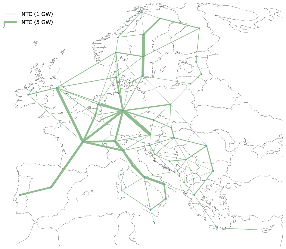
The Electricity reference grid in the PyPSA model was implemented as HVAC lines that neglect KVL and only model net transfer capacities (NTCs).

This is referred to as a Transport Model.

In PyPSA, this can be represented by the link component with carrier set to ‘DC’.

Let’s have a look at those links:

reference_grid_elec = n2.links.query("carrier == 'DC'")
reference_grid_elec.head()

	bus0	bus1	type	carrier	efficiency	active	build_year	lifetime	p_nom	p_nom_mod	...	voltage	dc	energy to power ratio	reversed	underwater_fraction	tags	bidirectional	location	length_original	geometry
Link
AL00-GR00-DC	AL00	GR00		DC	1.0	True	0	inf	600.0	0.0	...	380.0	1.0	NaN	False	0.0	AL00 -> GR00	NaN		219.635111	LINESTRING (20.036883988642362 41.117587702511...
AL00-ME00-DC	AL00	ME00		DC	1.0	True	0	inf	400.0	0.0	...	380.0	1.0	NaN	False	0.0	AL00 -> ME00	NaN		189.342890	LINESTRING (20.036883988642362 41.117587702511...
AL00-MK00-DC	AL00	MK00		DC	1.0	True	0	inf	500.0	0.0	...	380.0	1.0	NaN	False	0.0	AL00 -> MK00	NaN		153.308707	LINESTRING (20.036883988642362 41.117587702511...
AL00-RS00-DC	AL00	RS00		DC	1.0	True	0	inf	250.0	0.0	...	380.0	1.0	NaN	False	0.0	AL00 -> RS00	NaN		351.420535	LINESTRING (20.036883988642362 41.117587702511...
AT00-CH00-DC	AT00	CH00		DC	1.0	True	0	inf	1200.0	0.0	...	380.0	1.0	NaN	False	0.0	AT00 -> CH00	NaN		502.028400	LINESTRING (14.822183225330722 47.668898155000...

5 rows × 52 columns

That’s a lot of information! Let’s filter out some useful attributes.

reference_grid_elec.loc[:, ["bus0", "bus1", "p_nom", "p_nom_opt", "length"]].head()

	bus0	bus1	p_nom	p_nom_opt	length
Link
AL00-GR00-DC	AL00	GR00	600.0	0.0	219.635111
AL00-ME00-DC	AL00	ME00	400.0	0.0	189.342890
AL00-MK00-DC	AL00	MK00	500.0	0.0	153.308707
AL00-RS00-DC	AL00	RS00	250.0	0.0	351.420535
AT00-CH00-DC	AT00	CH00	1200.0	0.0	502.028400

You can observe that the p_nom_opt is not defined yet as this model was not solved yet.

You can narrow down to a specific country.

(
    reference_grid_elec.loc[:, ["bus0", "bus1", "p_nom", "p_nom_opt", "length"]].query(
        "Link.str.contains('ES')"
    )
)

	bus0	bus1	p_nom	p_nom_opt	length
Link
ES00-FR00-DC	ES00	FR00	5000.0	0.0	818.531610
ES00-PT00-DC	ES00	PT00	4200.0	0.0	469.515817
FR00-ES00-DC	FR00	ES00	5000.0	0.0	818.531610
PT00-ES00-DC	PT00	ES00	3500.0	0.0	469.515817

The model implements NTCs as unidirectional links. Electricity flows from bus0 (source) to bus1 (sink).

With the capacitiy p_nom and the length, we can also compute the total transmission capacity of the system in TWkm:

total_TWkm = (
    reference_grid_elec.p_nom.div(1e6)  # convert from PyPSA's base unit MW to TW
    .mul(reference_grid_elec.length)  # convert to TWkm
    .sum()
    .round(2)
)
print(
    f"Total electricity reference grid has a transmission capacity of {total_TWkm} TWkm."
)

Total electricity reference grid has a transmission capacity of 155.52 TWkm.

We can also check some individual number for specific connections using the .query() or the .filter(like='<your-filter>') method. .filter has the limitation to only work on indexes and column names.

# example
# `query()`
print(reference_grid_elec.query("Link.str.contains('DE00-BE00')").p_nom)  # in MW
# or `filter()`
print(reference_grid_elec.filter(like="DE00-BE00", axis=0).p_nom)

Link
DE00-BE00-DC    1000.0
Name: p_nom, dtype: float64
Link
DE00-BE00-DC    1000.0
Name: p_nom, dtype: float64

Exercise 2: Exploring the Electricity reference grid

Task a): Extract and filter for specific capacity information from your home country and compare with your data about these connections

Task b): Create a table with the import transmission capacity for each bidding zone (Advanced task: do the same for each country instead)

Task c): Which bidding zone / country has the largest total?

Hint: use pandas groupby method

# Your solution a)

# Your solution b)

# Your solution c)

Plotting the Electricity reference grid

Additionally, we can also use PyPSA’s built in interactive n.plot.explore() function to explore the electricity reference grid:

# create a copy of the network which only includes electricity
n_elec_grid = n2.copy()
n_elec_grid.remove(
    "Bus", n_elec_grid.buses.query("carrier != 'AC' or Bus.str.contains('DRES')").index
)

# explore the reference grid
n_elec_grid.plot.explore()

INFO:pypsa.plot.maps.interactive:Omitting 2121 links due to missing coordinates.

INFO:pypsa.plot.maps.interactive:Components rendered on the map: Bus, Link.

INFO:pypsa.plot.maps.interactive:Components omitted as they are missing or not selected: Generator, Line, Load, StorageUnit, Transformer.

Make this Notebook Trusted to load map: File -> Trust Notebook

We can also statically plot the electricity grid by utilizing a handy plotting function:

def plot_electricity_reference_grid(n, proj, lw_factor=1e3, figsize=(12, 12)):
    fig, ax = plt.subplots(figsize=figsize, subplot_kw={"projection": proj})
    n.plot.map(
        ax=ax,
        margin=0.06,
        link_widths=n.links.p_nom / lw_factor,
        link_colors="darkseagreen",
    )

    if not n.links.empty:
        sizes_ntc = [1, 5]
        labels_ntc = [f"NTC ({s} GW)" for s in sizes_ntc]
        scale_ntc = 1e3 / lw_factor
        sizes_ntc = [s * scale_ntc for s in sizes_ntc]

        legend_kw_dc = dict(
            loc=[0.0, 0.9],
            frameon=False,
            labelspacing=0.5,
            handletextpad=1,
            fontsize=13,
        )

        add_legend_lines(
            ax,
            sizes_ntc,
            labels_ntc,
            patch_kw=dict(color="darkseagreen"),
            legend_kw=legend_kw_dc,
        )

    plt.show()


def load_projection(plotting_params):
    proj_kwargs = plotting_params.get("projection", dict(name="EqualEarth"))
    proj_func = getattr(ccrs, proj_kwargs.pop("name"))
    return proj_func(**proj_kwargs)


proj = load_projection(dict(name="EqualEarth"))

plot_electricity_reference_grid(n_elec_grid, proj)

/opt/hostedtoolcache/Python/3.11.11/x64/lib/python3.11/site-packages/cartopy/io/__init__.py:241: DownloadWarning:

Downloading: https://naturalearth.s3.amazonaws.com/50m_cultural/ne_50m_admin_0_boundary_lines_land.zip

/opt/hostedtoolcache/Python/3.11.11/x64/lib/python3.11/site-packages/cartopy/io/__init__.py:241: DownloadWarning:

Downloading: https://naturalearth.s3.amazonaws.com/50m_physical/ne_50m_coastline.zip

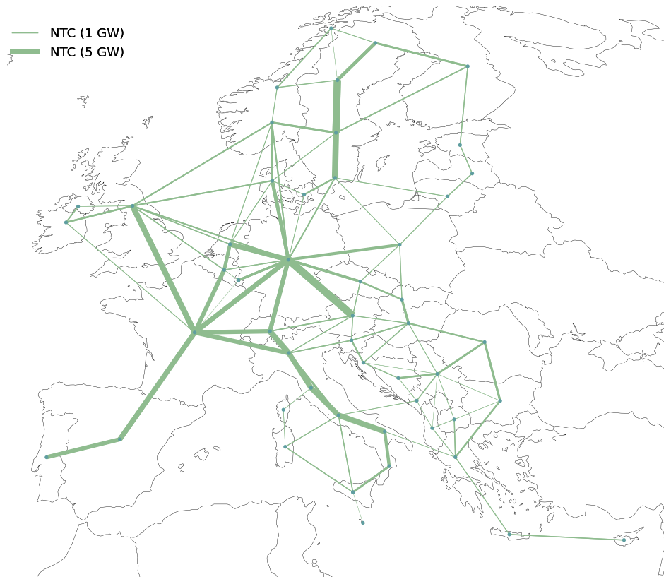
You’ve just created the reference grid published in the Scenarios Methodology report from TYNDP 2024!

Exercise 3: Plotting the Electricity reference grid

Task a): How would you change an NTC value in the reference grid?

!Hint: You can use the .loc operator

Task b): How would add a new candidate to the reference grid? Choose one, add it to your network and plot the new network to verify

!Hint: You can have a look at our minimal example from above and at the parameters of already included links for inspiration

# Your solution a)

# Your solution b)

Explore the Hydrogen reference grid

Similar to the Electricity reference grid, the H2 reference grid in the PyPSA model was implemented using the link component to represent the transport model of the Scenario Building.

Let’s have a look at those Hydrogen reference grid links:

reference_grid_h2 = n2.links.query("carrier == 'H2 pipeline'")
reference_grid_h2.head()

	bus0	bus1	type	carrier	efficiency	active	build_year	lifetime	p_nom	p_nom_mod	...	voltage	dc	energy to power ratio	reversed	underwater_fraction	tags	bidirectional	location	length_original	geometry
Link
H2 pipeline AT -> DE	AT H2 Z2	DE H2 Z2		H2 pipeline	1.0	True	0	50.0	6250.0	0.0	...	NaN	NaN	NaN	False	NaN		0.0		768.287118
H2 pipeline AT -> IBIT	AT H2 Z2	IBIT H2 Z2		H2 pipeline	1.0	True	0	50.0	5250.0	0.0	...	NaN	NaN	NaN	False	NaN		0.0		694.620395
H2 pipeline AT -> SI	AT H2 Z2	SI H2 Z2		H2 pipeline	1.0	True	0	50.0	0.0	0.0	...	NaN	NaN	NaN	False	NaN		0.0		247.449222
H2 pipeline AT -> SK	AT H2 Z2	SK H2 Z2		H2 pipeline	1.0	True	0	50.0	6000.0	0.0	...	NaN	NaN	NaN	False	NaN		0.0		469.275999
H2 pipeline BE -> DE	BE H2 Z2	DE H2 Z2		H2 pipeline	1.0	True	0	50.0	3790.0	0.0	...	NaN	NaN	NaN	False	NaN		0.0		552.792303

5 rows × 52 columns

Again, it’s a lot of information! Let’s filter out some useful attributes.

reference_grid_h2.loc[:, ["bus0", "bus1", "p_nom", "p_nom_opt", "length"]].head()

	bus0	bus1	p_nom	p_nom_opt	length
Link
H2 pipeline AT -> DE	AT H2 Z2	DE H2 Z2	6250.0	0.0	768.287118
H2 pipeline AT -> IBIT	AT H2 Z2	IBIT H2 Z2	5250.0	0.0	694.620395
H2 pipeline AT -> SI	AT H2 Z2	SI H2 Z2	0.0	0.0	247.449222
H2 pipeline AT -> SK	AT H2 Z2	SK H2 Z2	6000.0	0.0	469.275999
H2 pipeline BE -> DE	BE H2 Z2	DE H2 Z2	3790.0	0.0	552.792303

Exercise 4: Exploring the Hydrogen reference grid

Let’s focus on interconnections between two specific countries.

Task a): Choose two countries and find the right H2 pipelines connecting the two

Hint: use pandas query method

Again, we can compute the total transmission capacity of the system in TWkm.

Task b): Without looking at the previous section, can you remember how to calculate this?

# Your solution a)

# Your solution b)

Plotting the Hydrogen reference grid

Again, we can also use PyPSA’s built in interactive n.plot.explore() function to explore the hydrogen reference grid.

As we can see, the spatial resolution of the H2 reference grid is different to the electricity reference grid.

# create a copy of the network which only includes electricity
n_h2_grid = n2.copy()
n_h2_grid.remove("Bus", n_h2_grid.buses.query("carrier != 'H2'").index)
n_h2_grid.remove("Link", n_h2_grid.links.query("p_nom == 0").index)

# explore the reference grid
n_h2_grid.plot.explore()

INFO:pypsa.plot.maps.interactive:Omitting 209 links due to missing coordinates.

INFO:pypsa.plot.maps.interactive:Components rendered on the map: Bus, Link.

INFO:pypsa.plot.maps.interactive:Components omitted as they are missing or not selected: Generator, Line, Load, StorageUnit, Transformer.

Make this Notebook Trusted to load map: File -> Trust Notebook

We can also plot the hydrogen grid by utilizing another handy plotting function:

def plot_h2_reference_grid(
    n,
    proj,
    lw_factor=4e3,
    figsize=(12, 12),
    color_h2_pipe="#499a9c",
    color_h2_node="#ff29d9",
):
    n = n.copy()

    n.links.drop(
        n.links.index[~n.links.carrier.str.contains("H2 pipeline")], inplace=True
    )
    h2_pipes = n.links[n.links.carrier == "H2 pipeline"].p_nom

    link_widths_total = h2_pipes / lw_factor
    if link_widths_total.notnull().empty:
        print("No base H2 pipeline capacities to plot.")
        return
    link_widths_total = link_widths_total.reindex(n.links.index).fillna(0.0)

    n.buses.drop(n.buses.index[~n.buses.carrier.str.contains("H2")], inplace=True)

    fig, ax = plt.subplots(figsize=figsize, subplot_kw={"projection": proj})

    n.plot.map(
        geomap=True,
        bus_sizes=0.1,
        bus_colors=color_h2_node,
        link_colors=color_h2_pipe,
        link_widths=link_widths_total,
        branch_components=["Link"],
        ax=ax,
    )

    sizes = [30, 10]
    labels = [f"{s} GW" for s in sizes]
    scale = 1e3 / 4e3
    sizes = [s * scale for s in sizes]

    legend_kw = dict(
        loc="upper left",
        bbox_to_anchor=(0.005, 1.1),
        frameon=False,
        ncol=2,
        labelspacing=0.8,
        handletextpad=1,
    )

    add_legend_lines(
        ax,
        sizes,
        labels,
        patch_kw=dict(color="lightgrey"),
        legend_kw=legend_kw,
    )

    legend_kw = dict(
        loc="upper left",
        bbox_to_anchor=(0.15, 1.13),
        labelspacing=0.8,
        handletextpad=0,
        frameon=False,
    )

    add_legend_circles(
        ax,
        sizes=[0.2],
        labels=["H2 Node"],
        srid=n.srid,
        patch_kw=dict(facecolor=color_h2_node),
        legend_kw=legend_kw,
    )

    legend_kw = dict(
        loc="upper left",
        bbox_to_anchor=(0, 1.13),
        ncol=1,
        frameon=False,
    )

    add_legend_patches(ax, [color_h2_pipe], ["H2 Pipeline"], legend_kw=legend_kw)

    ax.set_facecolor("white")

    plt.show()

plot_h2_reference_grid(n_h2_grid, proj)

/opt/hostedtoolcache/Python/3.11.11/x64/lib/python3.11/site-packages/pypsa/plot/maps/static.py:1678: UserWarning:

When combining n.plot() with other plots on a geographical axis, ensure n.plot() is called first or the final axis extent is set initially (ax.set_extent(boundaries, crs=crs)) for consistent legend circle sizes.

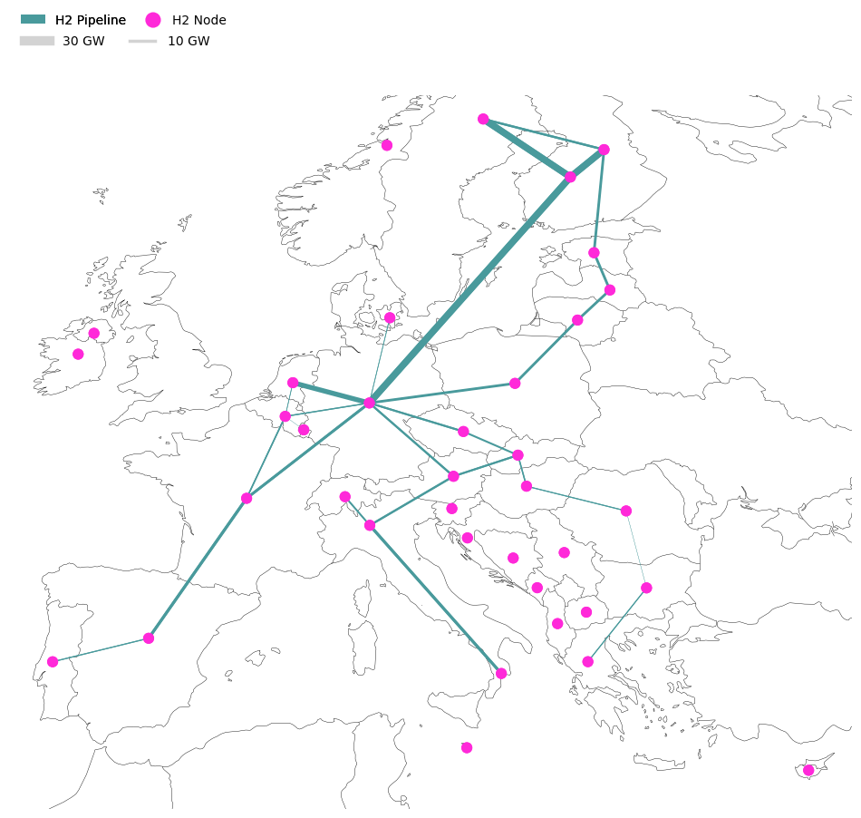
You’ve just created the hydrogen reference grid published in the Scenarios Methodology report from TYNDP 2024!

Exercise 5: Reference grid coupling in Italy

As you know, the geographical resolution of the electricity and hydrogen grids are different.

Take some time to verify the coupling between electricity and hydrogen in Italy.

# Your solution

Extracting insights & Visualization

Import the solved model

n3 = pypsa.Network("post-network.nc")

INFO:pypsa.io:Imported network post-network.nc has buses, carriers, generators, global_constraints, links, loads, shapes, storage_units, stores

Extract insights from the network using PyPSA.statistics

Let’s investigate the results from the solved model. For convenience, let’s save the accessor in a variable.

The full API documentation is available in pypsa documentation.

s = n3.statistics

You can easily have an comprehensive overview of the system level results.

s().head()

		Optimal Capacity	Installed Capacity	Supply	Withdrawal	Energy Balance	Transmission	Capacity Factor	Curtailment	Capital Expenditure	Operational Expenditure	Revenue	Market Value
Generator	Offshore Wind (AC)	59667.63846	6580.28372	2.336326e+08	0.0	2.336326e+08	0.0	0.446983	1.628091e+07	1.206196e+10	5.772445e+06	1.371072e+10	58.684940
	Offshore Wind (DC)	79517.60138	13350.65347	3.836668e+08	0.0	3.836668e+08	0.0	0.550791	7.110183e+06	1.832538e+10	9.456484e+06	2.127265e+10	55.445638
	Offshore Wind (Floating)	26188.43674	5074.35608	1.057571e+08	0.0	1.057571e+08	0.0	0.460994	9.206199e+05	6.145530e+09	2.566804e+06	5.906603e+09	55.850669
	Onshore Wind	313677.75700	184845.68700	7.470741e+08	0.0	7.470741e+08	0.0	0.271879	1.783103e+07	3.629873e+10	1.861170e+07	3.442422e+10	46.078722
	Run of River	47774.12902	47774.12902	1.704413e+08	0.0	1.704413e+08	0.0	0.407266	3.359915e+04	1.472257e+10	1.700200e+06	1.066173e+10	62.553712

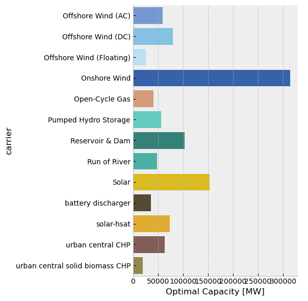
Let’s have a look to optimal renewable capacities.

(
    s.optimal_capacity(
        bus_carrier=["AC", "low voltage"],
        comps="Generator",
    ).div(
        1e3
    )  # GW
)

carrier
Offshore Wind (AC)           59.667638
Offshore Wind (DC)           79.517601
Offshore Wind (Floating)     26.188437
Onshore Wind                313.677757
Run of River                 47.774129
Solar                       152.958181
solar rooftop               694.672489
solar-hsat                   73.592653
dtype: float64

You can get it as fancy as you want!

(
    s.optimal_capacity(
        bus_carrier=["AC", "low voltage"],
        groupby=["location", "carrier"],
        comps="Generator",
    )
    .div(1e3)  # GW
    .to_frame(name="p_nom_opt")
    .pivot_table(index="location", columns="carrier", values="p_nom_opt")
    .fillna(0)
    .assign(Total=lambda df: df.sum(axis=1))
    .sort_values(by="Total", ascending=False)
    .round(2)
).head()

carrier	Offshore Wind (AC)	Offshore Wind (DC)	Offshore Wind (Floating)	Onshore Wind	Run of River	Solar	solar rooftop	solar-hsat	Total
location
DE00	4.24	21.70	0.53	56.42	4.76	53.67	80.41	0.00	221.73
FR00	27.60	6.91	21.12	17.48	6.51	11.06	122.71	0.00	213.39
GB00	8.61	3.28	3.57	81.05	2.87	12.52	42.45	0.00	154.36
ES00	0.00	0.00	0.00	26.81	0.28	10.14	84.74	29.85	151.83
PL00	5.17	5.81	0.00	19.71	0.18	3.95	37.31	0.00	72.13

Task: Take some time and try to fine tune this query to your needs

We can also easily look into the energy balance for a specific carrier by Node.

So, let’s investigate the Hydrogen balance at the Z1 and Z2 nodes of Germany (DE):

df = (
    s.energy_balance(groupby=["bus_carrier", "country", "bus", "carrier", "name"])
    .div(1e6)  # TWh
    .to_frame(name="Balance [TWh]")
    .query(
        "(bus_carrier.str.contains('Hydrogen')) "
        "and (country == 'DE') "
        " and (abs(`Balance [TWh]`) > 1e-2)"
    )
    .round(2)
)
df

						Balance [TWh]
component	bus_carrier	country	bus	carrier	name
Load	Hydrogen Storage	DE	DE H2 Z2	H2 for industry	DE00 H2 Z2 for industry	-17.46
Link	Hydrogen Storage	DE	DE H2 Z1	H2 pipeline	H2 pipeline DEH2Z1 -> DEH2Z2	-24.18
				SMR CC	DE H2 Z1 SMR CC	24.18
			DE H2 Z2	H2 pipeline	H2 pipeline DE -> AT	-1.72
					H2 pipeline DE -> CZ	-0.18
					H2 pipeline DE -> FR	-0.07
					H2 pipeline DE -> IBFI	-0.97
					H2 pipeline DE -> PL	-21.63
					H2 pipeline DEH2Z1 -> DEH2Z2	24.18
					H2 pipeline DK -> DE	13.88
					H2 pipeline FR -> DE	2.59
					H2 pipeline NL -> DE	1.39

# verify energy balance
df.groupby(by="bus").sum()

	Balance [TWh]
bus
DE H2 Z1	0.00
DE H2 Z2	0.01

exports = df.query("name.str.contains('DE ->')")
export_twh = exports["Balance [TWh]"].sum().round(2)
print(f"DE exports {export_twh} TWh of H2.")

imports = df.query(
    "(name.str.contains('-> DE')) and not (name.str.contains('Z1')) and not (name.str.contains('Z2'))"
)
import_twh = imports["Balance [TWh]"].sum().round(2)
print(f"DE imports {import_twh} TWh of H2.")

balance_twh = import_twh + export_twh
print(
    f"DE is a net {'importer' if balance_twh > 0 else 'exporter'} ({balance_twh.round(2)} TWh)."
)

DE exports -24.57 TWh of H2.
DE imports 17.86 TWh of H2.
DE is a net exporter (-6.71 TWh).

… or look at renewable curtailment in the system:

(
    s.curtailment(
        bus_carrier=["AC", "low voltage"],
        groupby=["location", "carrier"],
    )
    .div(1e6)  # TWh
    .to_frame(name="p_nom_opt")
    .pivot_table(index="location", columns="carrier", values="p_nom_opt")
    .fillna(0)
    .assign(Total=lambda df: df.sum(axis=1))
    .sort_values(by="Total", ascending=False)
    .round(2)
).head()

carrier	Offshore Wind (AC)	Offshore Wind (DC)	Offshore Wind (Floating)	Onshore Wind	Pumped Hydro Storage	Reservoir & Dam	Run of River	Solar	solar rooftop	solar-hsat	Total
location
ES00	0.00	0.00	0.00	2.75	84.42	98.52	0.0	0.01	3.22	3.35	192.28
CH00	0.00	0.00	0.00	0.00	48.19	68.73	0.0	0.05	0.36	0.04	117.37
NOS0	0.00	0.00	0.00	0.00	1.53	113.26	0.0	0.00	0.00	0.00	114.79
FR00	5.61	0.93	0.61	0.57	40.16	27.26	0.0	0.01	0.99	0.00	76.15
AT00	0.00	0.00	0.00	0.01	50.25	20.30	0.0	0.01	0.15	0.30	71.02

Task: Explore the pypsa documentation and try this out yourself

Visualizing results using PyPSA.statistics

The PyPSA.statistics module can also be used to create some really handy static plotting to investigate the results of a model.

# let's fill missing colors first
n3.carriers.loc["none", "color"] = "#000000"
n3.carriers.loc["", "color"] = "#000000"

Let’s now plot the optimal renewable capacities that we investigated before.

s.optimal_capacity.plot.bar(
    bus_carrier="AC",
    query="value>1e3",
    height=6,
);

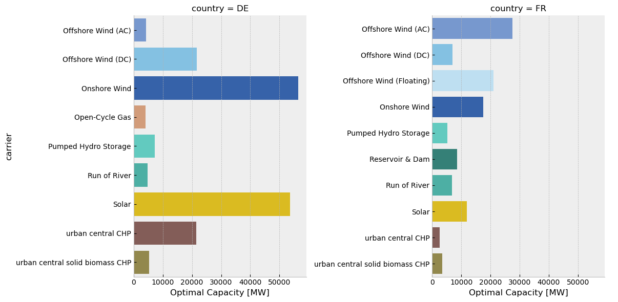
You can also have details for specific countries.

s.optimal_capacity.plot.bar(
    bus_carrier="AC",
    query="value>1e3 and country in ['DE', 'FR']",
    height=6,
    facet_col="country",
);

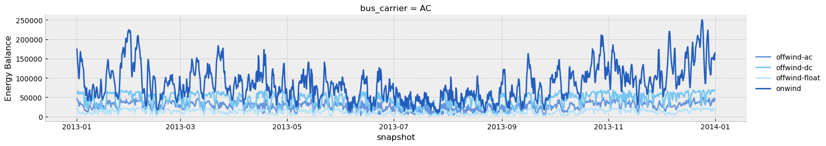
You can have a closer look to the wind production

s.energy_balance.plot.line(
    facet_row="bus_carrier",
    y="value",
    x="snapshot",
    carrier="wind",
    nice_names=False,
    color="carrier",
    aspect=5.0,
);

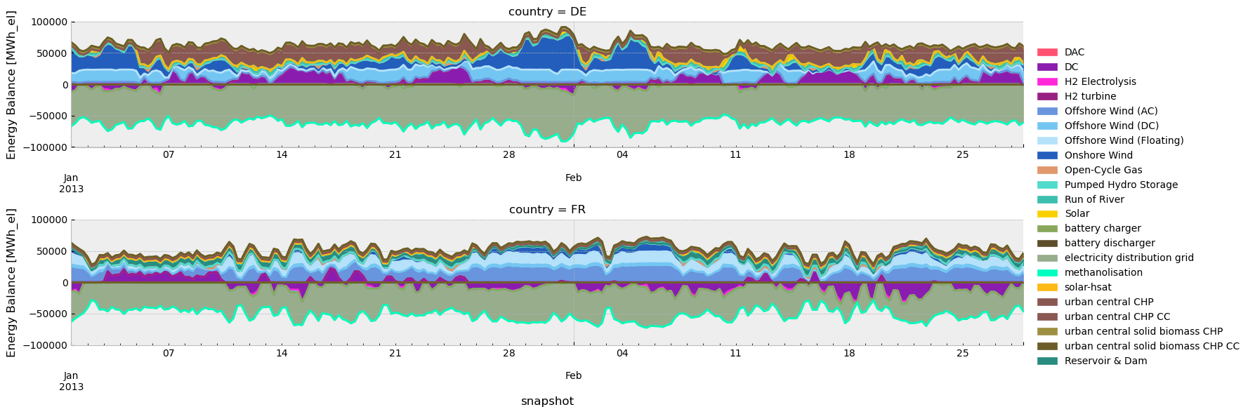
… or to the dispatch for specific countries.

s.energy_balance.plot.area(
    bus_carrier=["AC"],
    y="value",
    x="snapshot",
    color="carrier",
    stacked=True,
    facet_row="country",
    query="country in ['DE', 'FR'] and snapshot < '2013-03'",
    aspect=5,
);

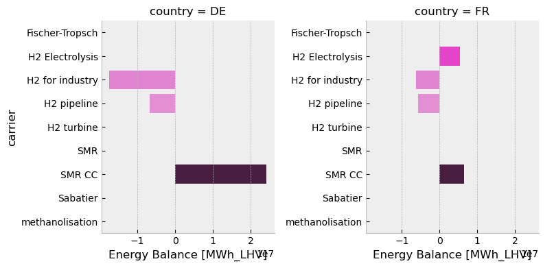
You can also explore H2 results.

s.energy_balance.plot.bar(
    bus_carrier=["H2"],
    y="carrier",
    x="value",
    color="carrier",
    facet_col="country",
    height=4,
    aspect=1,
    query="country in ['DE', 'FR']",
);

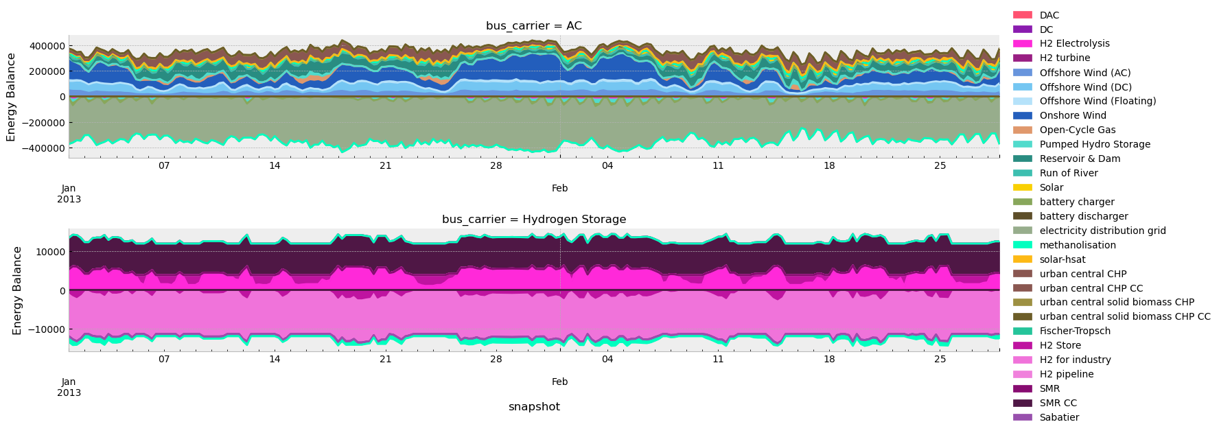
You can also explore the correlation between renewable production and hydrogen.

s.energy_balance.plot.area(
    bus_carrier=["AC", "H2"],
    y="value",
    x="snapshot",
    color="carrier",
    stacked=True,
    facet_row="bus_carrier",
    sharex=False,
    sharey=False,
    query="snapshot < '2013-03'",
    aspect=5,
);

WARNING:pypsa.descriptors:Multiple units found for carrier ['AC', 'H2']: ['MWh_el' 'MWh_LHV']

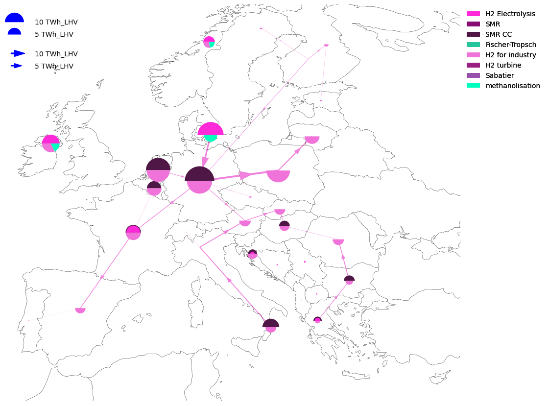
There is also the possibility to explore maps.

subplot_kw = {"projection": proj}
fig, ax = plt.subplots(figsize=(12, 12), subplot_kw=subplot_kw)
s.energy_balance.plot.map(
    bus_carrier="H2",
    ax=ax,
    bus_area_fraction=0.007,
    flow_area_fraction=0.004,
    legend_circles_kw=dict(
        frameon=False,
        labelspacing=0.8,
        handletextpad=1.5,
    ),
    legend_arrows_kw=dict(
        frameon=False,
        labelspacing=0.8,
        handletextpad=1.5,
    ),
);

/opt/hostedtoolcache/Python/3.11.11/x64/lib/python3.11/site-packages/pypsa/plot/maps/static.py:1738: UserWarning:

When combining n.plot() with other plots on a geographical axis, ensure n.plot() is called first or the final axis extent is set initially (ax.set_extent(boundaries, crs=crs)) for consistent legend semicircle sizes.

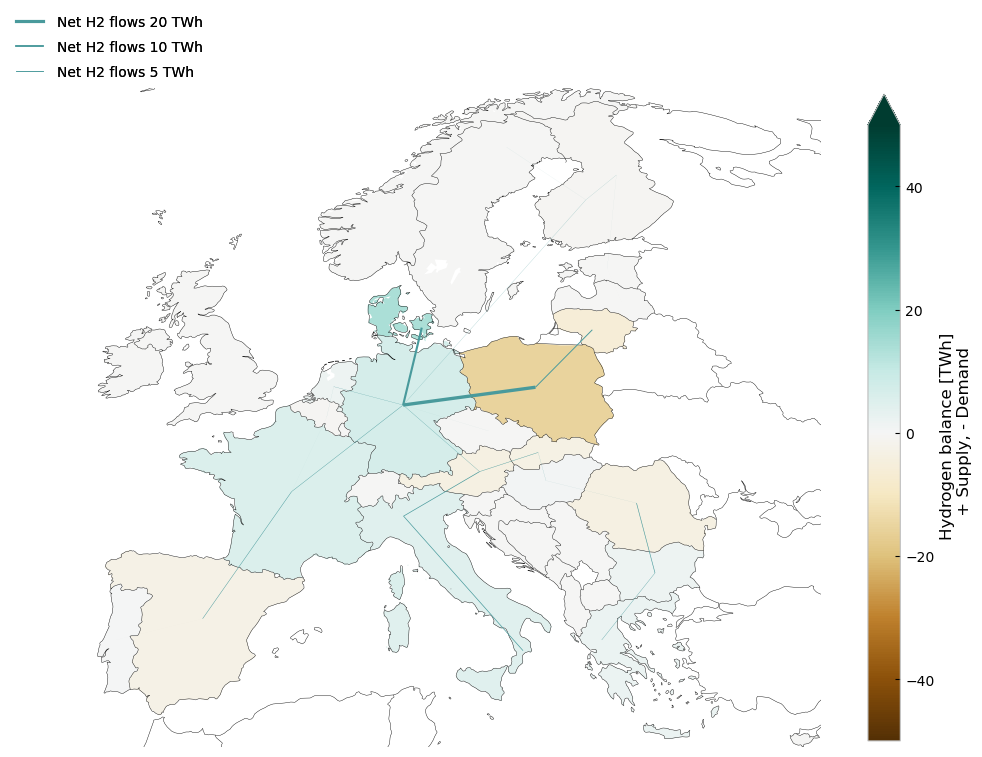
But, to get something neat, you might need to code it yourself. Indeed, with some tweaking and construction, we can use PyPSA’s plotting to create some really cool visualizations of the resulting net hydrogen flows in the network.

def plot_net_H2_flows(n, regions, countries=[], figsize=(12, 12)):
    network = n.copy()
    if "H2 pipeline" not in n.links.carrier.unique():
        return
    if len(countries) == 0:
        countries = regions.index.values

    linewidth_factor = 9e6
    # MW below which not drawn
    line_lower_threshold = 1e2
    min_energy = 0
    lim = 50
    link_color = "#499a9c"
    flow_factor = 100

    # get H2 energy balance per node
    carrier = "H2"
    h2_energy_balance = network.statistics.energy_balance(
        bus_carrier="H2", comps=["Link", "Load"], groupby=["country", "carrier"]
    ).to_frame()

    to_drop = ["H2 pipeline"]
    # drop pipelines and storages from energy balance
    h2_energy_balance.drop(h2_energy_balance.loc[:, :, to_drop, :].index, inplace=True)
    # filter for countries
    h2_energy_balance = h2_energy_balance.loc[:, countries, :, :]
    regions = regions.loc[countries]

    regions["H2"] = h2_energy_balance.groupby("country").sum().div(1e6)  # TWh

    # Drop non-hydrogen buses so they don't clutter the plot
    # And filter for countries
    network.buses.drop(network.buses.query("carrier != 'H2'").index, inplace=True)
    network.buses.drop(
        network.buses.query("country not in @countries").index, inplace=True
    )

    # drop all links which are not H2 pipelines
    network.links.drop(
        network.links.index[~network.links.carrier.str.contains("H2 pipeline")],
        inplace=True,
    )

    network.links["flow"] = network.snapshot_weightings.generators @ network.links_t.p0

    positive_order = network.links.bus0 < network.links.bus1
    swap_buses = {"bus0": "bus1", "bus1": "bus0"}
    network.links.loc[~positive_order] = network.links.rename(columns=swap_buses)
    network.links.loc[~positive_order, "flow"] = -network.links.loc[
        ~positive_order, "flow"
    ]
    network.links.index = network.links.apply(
        lambda x: f"H2 pipeline {x.bus0} -> {x.bus1}", axis=1
    )
    network.links = network.links.groupby(network.links.index).agg(
        dict(flow="sum", bus0="first", bus1="first", carrier="first", p_nom_opt="sum")
    )
    network.links.flow = network.links.flow.where(network.links.flow.abs() > min_energy)

    # drop links not connecting countries in country list
    network.links.drop(
        network.links.loc[
            (
                (~network.links.bus0.str.contains("|".join(countries)))
                | (~network.links.bus1.str.contains("|".join(countries)))
            )
        ].index,
        inplace=True,
    )

    proj = ccrs.EqualEarth()
    coords = regions.get_coordinates()
    map_opts["boundaries"] = [
        x for y in zip(coords.min().values, coords.max().values) for x in y
    ]
    regions = regions.to_crs(proj.proj4_init)

    fig, ax = plt.subplots(figsize=figsize, subplot_kw={"projection": proj})

    link_widths_flows = network.links.flow.div(linewidth_factor).fillna(0)

    network.plot.map(
        geomap=True,
        bus_sizes=0,
        link_colors=link_color,
        link_widths=link_widths_flows,
        branch_components=["Link"],
        ax=ax,
        flow=pd.concat({"Link": link_widths_flows * flow_factor}),
        **map_opts,
    )

    regions.plot(
        ax=ax,
        column="H2",
        cmap="BrBG",
        linewidths=0,
        legend=True,
        vmax=lim,
        vmin=-lim,
        legend_kwds={
            "label": "Hydrogen balance [TWh] \n + Supply, - Demand",
            "shrink": 0.7,
            "extend": "max",
        },
    )

    legend_kw = dict(
        loc="upper left",
        bbox_to_anchor=(-0.1, 1.13),
        frameon=False,
        labelspacing=0.8,
        handletextpad=1,
    )

    sizes = [20, 10, 5]
    labels = [f"Net H2 flows {s} TWh" for s in sizes]
    scale = 1e6 / linewidth_factor
    sizes = [s * scale for s in sizes]
    add_legend_lines(
        ax,
        sizes,
        labels,
        patch_kw=dict(color=link_color),
        legend_kw=legend_kw,
    )

    ax.set_facecolor("white")


map_opts = {
    "boundaries": [-11, 30, 34, 71],
    "geomap_colors": {
        "ocean": "white",
        "land": "white",
    },
}

h2_regions = bz.dissolve(by="country")
plot_net_H2_flows(n3, h2_regions)

/opt/hostedtoolcache/Python/3.11.11/x64/lib/python3.11/site-packages/pypsa/plot/maps/static.py:1370: DeprecationWarning:

The `flow` argument is deprecated, use `line_flow`, `link_flow` and `transformer_flow` instead. Multiindex Series are not supported anymore.

/opt/hostedtoolcache/Python/3.11.11/x64/lib/python3.11/site-packages/cartopy/io/__init__.py:241: DownloadWarning:

Downloading: https://naturalearth.s3.amazonaws.com/50m_physical/ne_50m_land.zip

/opt/hostedtoolcache/Python/3.11.11/x64/lib/python3.11/site-packages/cartopy/io/__init__.py:241: DownloadWarning:

Downloading: https://naturalearth.s3.amazonaws.com/50m_physical/ne_50m_ocean.zip

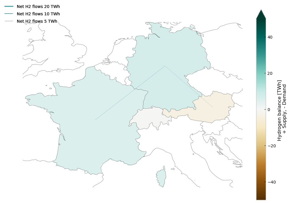
Or, if you want to zoom on specific countries.

plot_net_H2_flows(n3, h2_regions, countries=["DE", "FR", "CH", "AT"])

/opt/hostedtoolcache/Python/3.11.11/x64/lib/python3.11/site-packages/pypsa/plot/maps/static.py:1370: DeprecationWarning:

The `flow` argument is deprecated, use `line_flow`, `link_flow` and `transformer_flow` instead. Multiindex Series are not supported anymore.

Task: Take some time to play around with the introduced plotting functions

Solutions

Exercise 1: Add another town to the model

Show code cell content Hide code cell content

n1.add("Bus", "Shelbyville", v_nom=380, carrier="AC")

Index(['Shelbyville'], dtype='object')

Show code cell content Hide code cell content

n1.add(
    "Link",
    "Springfield <-> Shelbyville",
    bus0="Springfield",
    bus1="Shelbyville",
    p_nom=10,
    carrier="AC",
    p_min_pu=-1,  # For bidirectional
)

Index(['Springfield <-> Shelbyville'], dtype='object')

Show code cell content Hide code cell content

n1.add(
    "Generator",
    "coal",
    carrier="AC",
    bus="Shelbyville",
    p_nom_extendable=False,
    marginal_cost=50,  # €/MWh
    p_nom=100,  # MW
)

Index(['coal'], dtype='object')

Show code cell content Hide code cell content

n1.add(
    "Load",
    "Small town 2",
    carrier="AC",
    bus="Shelbyville",
    p_set=70,  # MW
)

Index(['Small town 2'], dtype='object')

Show code cell content Hide code cell content

n1.loads

	bus	carrier	type	p_set	q_set	sign	active
Load
Small town	Springfield	AC		120.0	0.0	-1.0	True
Small town 2	Shelbyville	AC		70.0	0.0	-1.0	True

Show code cell content Hide code cell content

n1.optimize(solver_name="highs")

---------------------------------------------------------------------------
KeyError                                  Traceback (most recent call last)
Cell In[80], line 1
----> 1 n1.optimize(solver_name="highs")

File /opt/hostedtoolcache/Python/3.11.11/x64/lib/python3.11/site-packages/pypsa/optimization/optimize.py:633, in OptimizationAccessor.__call__(self, *args, **kwargs)
    631 @wraps(optimize)
    632 def __call__(self, *args: Any, **kwargs: Any) -> Any:
--> 633     return optimize(self.n, *args, **kwargs)

File /opt/hostedtoolcache/Python/3.11.11/x64/lib/python3.11/site-packages/pypsa/optimization/optimize.py:593, in optimize(n, snapshots, multi_investment_periods, transmission_losses, linearized_unit_commitment, model_kwargs, extra_functionality, assign_all_duals, solver_name, solver_options, compute_infeasibilities, **kwargs)
    590 n._multi_invest = int(multi_investment_periods)
    591 n._linearized_uc = linearized_unit_commitment
--> 593 n.consistency_check(strict=["unknown_buses"])
    594 m = create_model(
    595     n,
    596     sns,
   (...)    601     **model_kwargs,
    602 )
    603 if extra_functionality:

File /opt/hostedtoolcache/Python/3.11.11/x64/lib/python3.11/site-packages/pypsa/consistency.py:859, in consistency_check(n, check_dtypes, strict)
    857 check_for_unknown_buses(n, c, "unknown_buses" in strict)
    858 check_for_unknown_carriers(n, c, "unkown_carriers" in strict)
--> 859 check_time_series(n, c, "time_series" in strict)
    860 check_static_power_attributes(n, c, "static_power_attrs" in strict)
    861 check_time_series_power_attributes(n, c, "time_series_power_attrs" in strict)

File /opt/hostedtoolcache/Python/3.11.11/x64/lib/python3.11/site-packages/pypsa/common.py:238, in deprecated_kwargs.<locals>.deco.<locals>.wrapper(*args, **kwargs)
    235 @functools.wraps(f)
    236 def wrapper(*args: Any, **kwargs: Any) -> Any:
    237     rename_kwargs(f.__name__, kwargs, aliases)
--> 238     return f(*args, **kwargs)

File /opt/hostedtoolcache/Python/3.11.11/x64/lib/python3.11/site-packages/pypsa/consistency.py:254, in check_time_series(n, component, strict)
    231 """
    232 Check if time series of component are aligned with network snapshots.
    233 
   (...)    251 
    252 """
    253 for attr in component.attrs.index[component.attrs.varying & component.attrs.static]:
--> 254     attr_df = component.dynamic[attr]
    256     diff = attr_df.columns.difference(component.static.index)
    257     if len(diff):

KeyError: 'efficiency4'

Show code cell content Hide code cell content

n1.objective

Show code cell content Hide code cell content

n1.generators_t.p

Show code cell content Hide code cell content

n1.buses_t.marginal_price

Show code cell content Hide code cell content

n1.links_t.p0

Exercise 2: Exploring the Electricity reference grid

Show code cell content Hide code cell content

# Solution a)
(reference_grid_elec.query("Link.str.contains('ES')")[["p_nom"]].div(1e3))  # in GW

Show code cell content Hide code cell content

# Solution b)
import_caps_bz = (
    reference_grid_elec.groupby("bus1")
    .p_nom.sum()
    .sort_values(ascending=False)
    .div(1e3)  # GW
)
import_caps_bz.head()

Show code cell content Hide code cell content

# Solution b) advanced
import_caps = (
    reference_grid_elec.assign(
        country_export=lambda x: x.bus0.str[:2], country_import=lambda x: x.bus1.str[:2]
    )
    .query("country_export != country_import")
    .groupby(by="country_import")
    .p_nom.sum()
    .sort_values(ascending=False)
    .div(1e3)  # GW
)
import_caps.head()

Show code cell content Hide code cell content

# Solution c)
# Bidding Zone
display(import_caps_bz.reset_index().iloc[0])
# Country
display(import_caps.reset_index().iloc[0])

Exercise 3: Plotting the Electricity reference grid

Show code cell content Hide code cell content

# Solution a)
n_elec_grid_ex = n_elec_grid.copy()
n_elec_grid_ex.links.loc["AL00-GR00-DC", "p_nom"] = 1000.00

Show code cell content Hide code cell content

# Solution b)
n_elec_grid_ex.add(
    "Link",
    "PL00-RO00-DC",
    bus0="PL00",
    bus1="RO00",
    carrier="DC",
    p_nom=600,
    p_nom_extendable=False,
    voltage=380.0,
    tags="PL00 -> RO00",
    length=230,
    capital_cost=25000,  # optional
)
plot_electricity_reference_grid(n_elec_grid_ex, proj)

Exercise 4: Exploring the Hydrogen reference grid

Show code cell content Hide code cell content

# Solution a)
(
    reference_grid_h2.query(
        "carrier.str.contains('H2') and Link.str.contains('DE') and Link.str.contains('BE')"
    )
)

Show code cell content Hide code cell content

# Solution b)
total_TWkm = (
    reference_grid_h2.p_nom.div(1e6)  # convert from PyPSA's base unit MW to TW
    .mul(reference_grid_h2.length)  # convert to TWkm
    .sum()
    .round(2)
)
print(f"Total H2 reference grid has a transmission capacity of {total_TWkm} TWkm.")

Exercise 5: Reference grid coupling in Italy

Show code cell content Hide code cell content

# IBIT node connects Italy with Austria and Switzerland.
(n2.links.query("carrier.str.contains('H2') and Link.str.contains('IBIT')"))

Show code cell content Hide code cell content

# IT node connects to electrolysers, H2 turbines and DRES capacities.
# IT node connects Italy with Spain and Slovenia.
(
    n2.links.query(
        "carrier.str.contains('H2') and Link.str.contains('IT') and not Link.str.contains('IBIT')"
    )
)