Workshop 3: Exploring NT Scenario Results, Modifying Assumptions, and Benchmarking

Note

At the end of this notebook, you will be able to:

1. Use PyPSA Explorer to analyze results

• Navigate and analyze NT scenario results using PyPSA-Explorer

• Compare 2030 and 2040 scenarios interactively

2. Benchmark Open-TYNDP against ENTSO-E TYNDP 2024

• Interpret differences between model outputs and TYNDP 2024 NT scenario

• Identify potential data inconsistencies, methodological differences, areas where Open-TYNDP can improve

3. Modify scenario assumptions

• Learn different ways how to change model assumptions and generate new scenario results

Note

If you have not set up Python on your computer, you can execute this tutorial in your browser via Google Colab. Click the rocket button in the top right corner and launch “Colab”. If that doesn’t work, download the .ipynb file and import it in Google Colab.

Then install the required packages by executing the following command in a Jupyter cell at the top of the notebook:

!pip install pypsa pypsa-explorer pandas matplotlib numpy pdf2image
!apt-get install poppler-utils

# uncomment for running this notebook on Colab
# !pip install pypsa pypsa-explorer pandas matplotlib numpy pdf2image
# !apt-get install poppler-utils

import os
from datetime import datetime
import pandas as pd
import pypsa
import shutil
import zipfile
from urllib.request import urlretrieve
from pdf2image import convert_from_path
from pdf2image.exceptions import PDFPageCountError
from IPython.display import Code, display
import matplotlib.pyplot as plt
from pypsa_explorer import create_app
from pathlib import Path

pypsa.options.params.statistics.round = 3
pypsa.options.params.statistics.drop_zero = True
pypsa.options.params.statistics.nice_names = False
plt.rcParams["figure.figsize"] = [14, 7]

def unzip_with_timestamps(zip_path, extract_to, keep_zip=True):
    """Unzip a file while preserving original file timestamps."""
    with zipfile.ZipFile(zip_path, "r") as zip_ref:
        for member in zip_ref.infolist():
            # Extract the file
            zip_ref.extract(member, extract_to)

            # Get the extracted file path
            extracted_path = os.path.join(extract_to, member.filename)

            # Get the modification time from the zip file
            date_time = datetime(*member.date_time)
            timestamp = date_time.timestamp()

            # Set both access and modification times
            os.utime(extracted_path, (timestamp, timestamp))
    if not keep_zip:
        os.remove(zip_path)

urls = {
    "data/results-1H-20251129.zip": "https://storage.googleapis.com/open-tyndp-data-store/workshop-03/results-1H-20251129.zip",
    "data/open-tyndp-20251129.zip": "https://storage.googleapis.com/open-tyndp-data-store/workshop-03/open-tyndp-20251129.zip",
    "scripts/_helpers.py": "https://raw.githubusercontent.com/open-energy-transition/open-tyndp-workshops/792b8474ab5096e5ab8db2822af4fcd9fe659eb6/open-tyndp-workshops/scripts/_helpers.py",
}

os.makedirs("data", exist_ok=True)
os.makedirs("scripts", exist_ok=True)
for name, url in urls.items():
    if os.path.exists(name):
        print(f"File {name} already exists. Skipping download.")
    else:
        print(f"Retrieving {name} from storage.")
        urlretrieve(url, name)
        print(f"File available in {name}.")

to_dir = "data/results-1H-20251129"
if not os.path.exists(to_dir):
    print(f"Unzipping data/results-1H-20251129.zip.")
    unzip_with_timestamps("data/results-1H-20251129.zip", "data/results-1H-20251129")
print(f"NT results available in '{to_dir}'.")

to_dir = "data/open-tyndp-20251129"
if not os.path.exists(to_dir):
    print(f"Unzipping data/open-tyndp-20251129.zip.")
    unzip_with_timestamps("data/open-tyndp-20251129.zip", "data/open-tyndp-20251129")
print(f"Open-TYNDP available in '{to_dir}'.")

print("Done")

Retrieving data/results-1H-20251129.zip from storage.

File available in data/results-1H-20251129.zip.
Retrieving data/open-tyndp-20251129.zip from storage.

File available in data/open-tyndp-20251129.zip.
File scripts/_helpers.py already exists. Skipping download.
Unzipping data/results-1H-20251129.zip.

NT results available in 'data/results-1H-20251129'.
Unzipping data/open-tyndp-20251129.zip.

Open-TYNDP available in 'data/open-tyndp-20251129'.
Done

1. Interactive Exploration with PyPSA-Explorer

PyPSA-Explorer is an interactive dashboard for visualizing and analyzing energy system networks. It provides:

• Energy balance analysis with both time series and aggregated views

• Capacity planning visualizations by technology and region

• Economic analysis showing CAPEX/OPEX breakdowns

• Interactive geographical network maps

• Support for visualising multiple networks

Let’s load the NT scenario results and explore them interactively.

# Load NT scenario networks for comparison
base_path = "data/results-1H-20251129/networks/"


def import_network(fn: str):
    n = pypsa.Network(fn)
    n.carriers.loc["none", "color"] = "#000000"
    return n


# Load networks directly into dictionary for PyPSA-Explorer
networks = {
    "NT 2030": import_network(base_path + "base_s_all___2030.nc"),
    "NT 2040": import_network(base_path + "base_s_all___2040.nc"),
}

WARNING:pypsa.network.io:Importing network from PyPSA version v1.0.4 while current version is v1.0.5. Read the release notes at `https://go.pypsa.org/release-notes` to prepare your network for import.

INFO:pypsa.network.io:Imported network 'PyPSA-Eur (tyndp)' has buses, carriers, generators, global_constraints, links, loads, shapes, storage_units, stores, sub_networks

WARNING:pypsa.network.io:Importing network from PyPSA version v1.0.4 while current version is v1.0.5. Read the release notes at `https://go.pypsa.org/release-notes` to prepare your network for import.

INFO:pypsa.network.io:Imported network 'PyPSA-Eur (tyndp)' has buses, carriers, generators, global_constraints, links, loads, shapes, storage_units, stores, sub_networks

PyPSA-Explorer can be launched in different ways depending on your environment:

• Local Jupyter: Use the terminal command (recommended) or inline display

• Google Colab: The dashboard launches inline, embedded directly in the notebook

Follow the instructions below for your specific environment.

# Detect if running on Google Colab
try:
    from google.colab import output

    IN_COLAB = True
    print(f"This notebook is running on Google Colab!")
except ImportError:
    IN_COLAB = False
    print(f"This notebook is running locally !")

port = 8050

This notebook is running locally !

For Local Users

If you’re running locally, we recommend launching PyPSA-Explorer from the terminal for optimal performance:

pypsa-explorer data/results-1H-20251129/networks/base_s_all___2030.nc:NT_2030 data/results-1H-20251129/networks/base_s_all___2040.nc:NT_2040

This command opens the dashboard in your default browser at http://localhost:8050.

Alternative: The cell below can launch the dashboard inline within the notebook, though the terminal method provides better performance and responsiveness.

# Terminal method recommended
USE_TERMINAL = True  # Change to False if you want to launch inline display

if not IN_COLAB and not USE_TERMINAL:
    # Local Jupyter: Inline display
    app = create_app(networks)
    app.run(jupyter_mode="tab", port=port, debug=False)

For Google Colab Users

Running PyPSA-Explorer on Google Colab requires a small workaround to display the dashboard properly inside the notebook.

First, let’s define a helper function to handle the setup:

def run_pypsa_explorer_in_colab(networks, port):
    print("Starting PyPSA Explorer for Google Colab...")

    # Create and start the app
    app = create_app(networks)

    import threading
    import time

    def run_server():
        app.run(jupyter_mode="external", port=port, debug=False)

    server_thread = threading.Thread(target=run_server, daemon=True)
    server_thread.start()

    # Wait for server to initialize
    time.sleep(5)
    print(f"✓ Server started on port {port}")

    # Display in iframe
    output.serve_kernel_port_as_iframe(port, height=1500)

if IN_COLAB:
    run_pypsa_explorer_in_colab(networks, port)

Tip for Colab users: To view the dashboard in fullscreen mode, click the three dots (⋮) in the top-right corner of the output cell and select “View output fullscreen”.

Using the Dashboard

Once the dashboard opens, you can explore these key features:

1. Energy Balance Tab

• View production, consumption, and storage patterns over time

• Switch between time series and aggregated views

• Filter by energy carrier (electricity, hydrogen, etc.)

• Filter by country or region

2. Capacity Tab

• Analyze installed capacities across scenarios

• Compare capacity buildout between 2030 and 2040

• View breakdowns by technology type and region

3. Economics Tab

• Examine costs and revenues

• Review CAPEX and OPEX breakdowns by technology

• Compare regional cost distributions

• Assess investment requirements

4. Network Map

• Visualize the geographical network layout

• View an interactive map with network components

• Zoom and pan to explore specific regions

Tip: Use the scenario selector buttons in the top-right corner to switch between NT 2030 and NT 2040 scenarios.

2. Benchmark Results

In Workshop 2, we introduced a benchmarking framework to systematically compare Open-TYNDP model outputs against the official TYNDP 2024 scenarios. This framework provides flexible and scalable validation across multiple metrics and methods, helping us to:

• Identify discrepancies: Compare demands, installed capacities, and generation volumes between model results and TYNDP targets

• Quantify differences: Calculate deviations by technology and investment year

• Guide improvements: Prioritize areas where the model requires refinement

Now, let’s apply this framework to our NT 2030 and 2040 scenario results to understand where the current model aligns with—or diverges from—TYNDP expectations.

First, we’ll define a helper function to visualize the benchmarks.

def show_benchmarks(
    fn: str,
    years: list = [2030, 2040],
    bench_path: str = "data/results-1H-20251129/validation/graphics_s_all___all_years",
):
    try:
        images = [
            convert_from_path(Path(bench_path, f"{fn}_{y}.pdf"))[0] for y in years
        ]
    except PDFPageCountError:
        print("File not found, skipping...")
        return

    fig, axes = plt.subplots(1, 2)
    for ax, img in zip(axes, images):
        ax.imshow(img)
        ax.axis("off")
    plt.tight_layout()
    plt.show()

Warning

Open-TYNDP is under active development and is not yet feature-complete. The current NT results presented below are preliminary results and several features still require improvement. These limitations must be understood when assessing the current benchmarking results.

When discussing the benchmarks, we can identify four categories of explanations for deviations from TYNDP 2024 reference values:

1. Data source discrepancies: Two data sources don’t seem to align, and the methodology is insufficient to derive the correct interpretation

2. Partial feature integration in Open-TYNDP: A specific feature must be expanded to appropriately reflect the TYNDP methodology

3. Scope discrepancies: The benchmarked and reference values use different scopes to report data (e.g., one uses EU27 while the other includes all modeled nodes)

4. Missing information or data: Default PyPSA-Eur values are used because the TYNDP assumptions have not yet been integrated

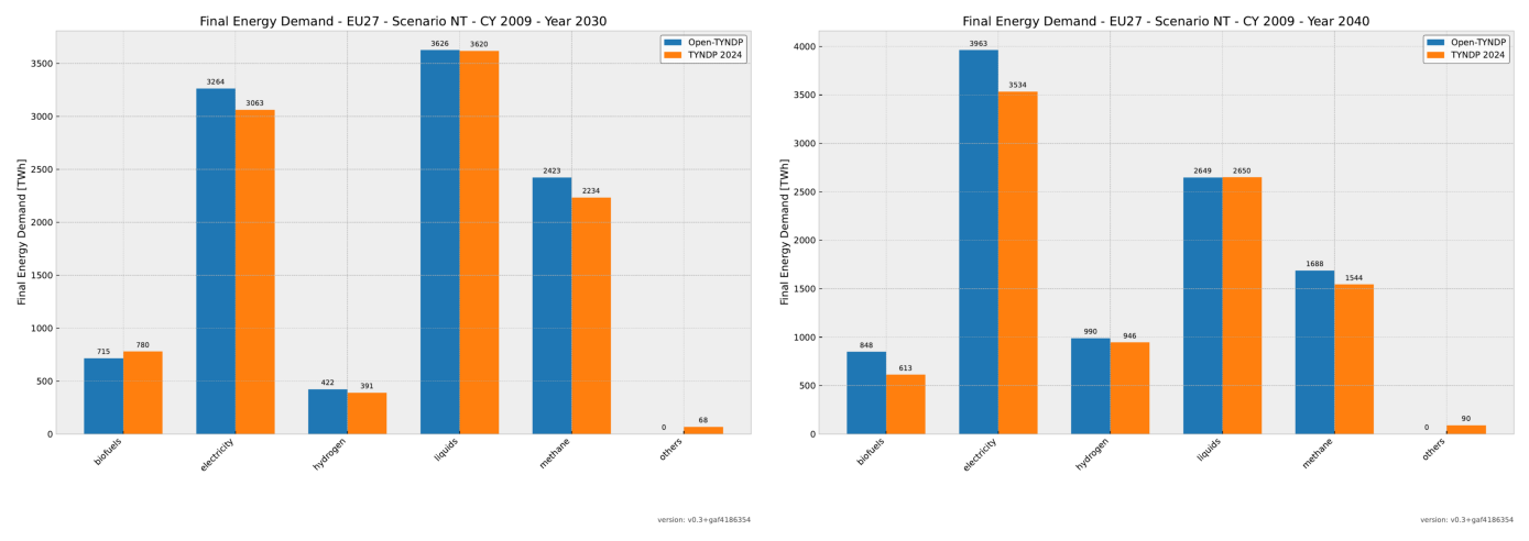
Final Energy Demand

Let’s examine each benchmark category in detail, starting with final energy demand across all carriers. We observe that demand for each carrier is now broadly reproduced. However, improvements are still needed to match the exact TYNDP post-processing methodology, and some discrepancies remain with exogenous inputs. Additionally, the benchmarked biofuels demand currently includes non-EU27 countries, which explains the larger value.

show_benchmarks("benchmark_final_energy_demand_eu27_cy2009")

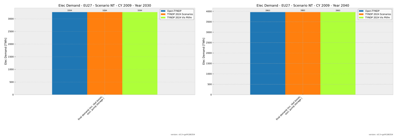
Electricity Demand

Electricity demand is an exogenous input to the model, taken directly from TYNDP 2024 data. Therefore, we achieve perfect alignment between the model input and TYNDP 2024 for this metric. Note, however, that the final electricity demand equals this exogenous input value, which differs from the reference value reported in TYNDP 2024.

show_benchmarks("benchmark_elec_demand_eu27_cy2009")

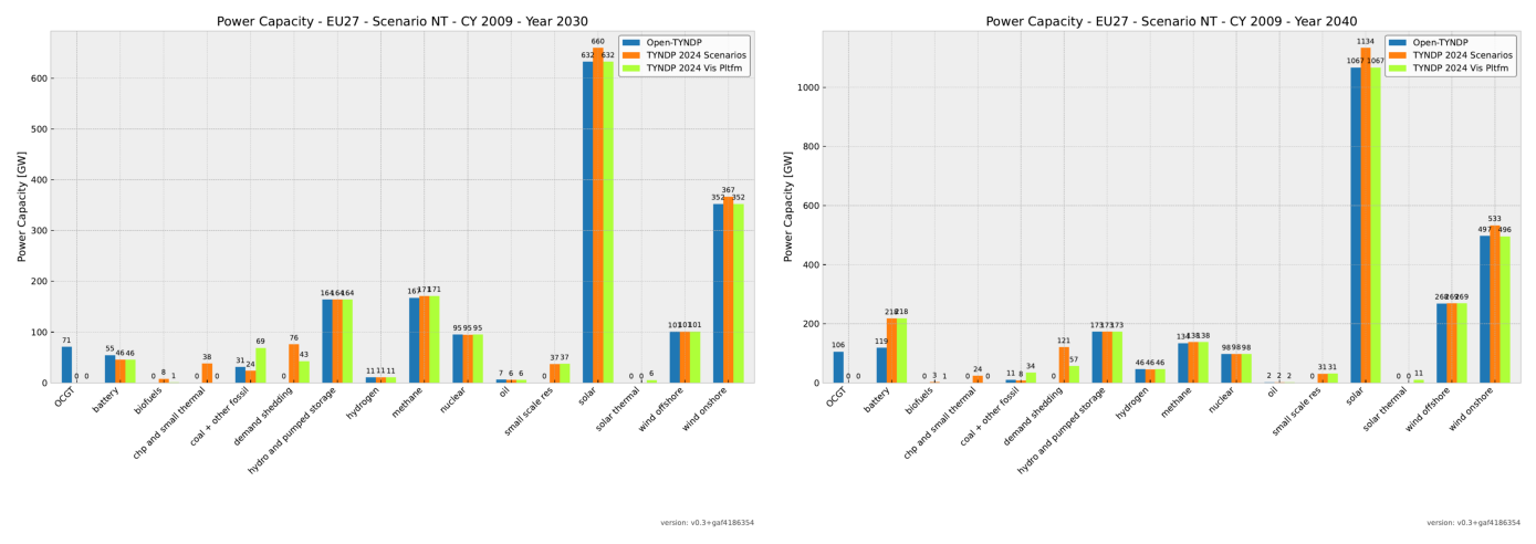
Power Capacities

Installed generation capacities are converging toward TYNDP 2024 values. Both renewable and conventional capacities have been fully integrated from the PEMMDB database. Open-TYNDP now closely reproduces TYNDP 2024 values, except for coal, where large discrepancies between data sources persist.

Some technologies still require implementation, including CHP and small thermal units, small-scale renewable energy systems, and solar thermal installations. Currently, OCGT units are retained in the system and used as peaking units because demand shedding has not yet been implemented in Open-TYNDP.

show_benchmarks("benchmark_power_capacity_eu27_cy2009")

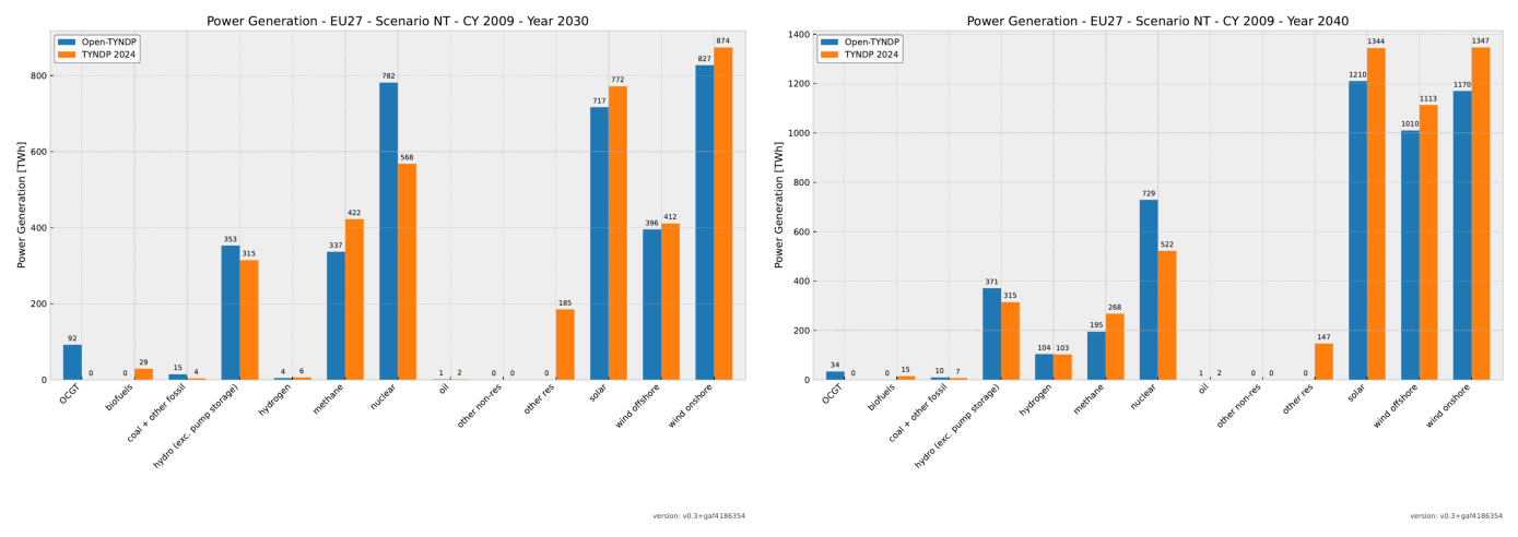
Electricity Generation

Actual electricity generation differs slightly from the TYNDP 2024 generation mix. Total generation values are closer to the reference but remain lower than reported values. As we’ll see later, lower power-to-gas (P2G) demand likely explains part of this difference. Additionally, electrical exchanges with non-modeled countries have not yet been integrated.

show_benchmarks("benchmark_power_generation_eu27_cy2009")

We can also explore the hourly time series energy balances in more detail.

networks["NT 2030"].statistics.energy_balance.iplot.area(
    bus_carrier=["AC", "H2"],
    y="value",
    x="snapshot",
    color="carrier",
    stacked=True,
    facet_row="bus_carrier",
    sharex=False,
    sharey=False,
    query="snapshot <= '2009-03-07' and snapshot >= '2009-03-01'",
)

WARNING:pypsa.network.descriptors:Multiple units found for carrier ['AC', 'H2']: ['MWh_el' 'MWh_LHV']

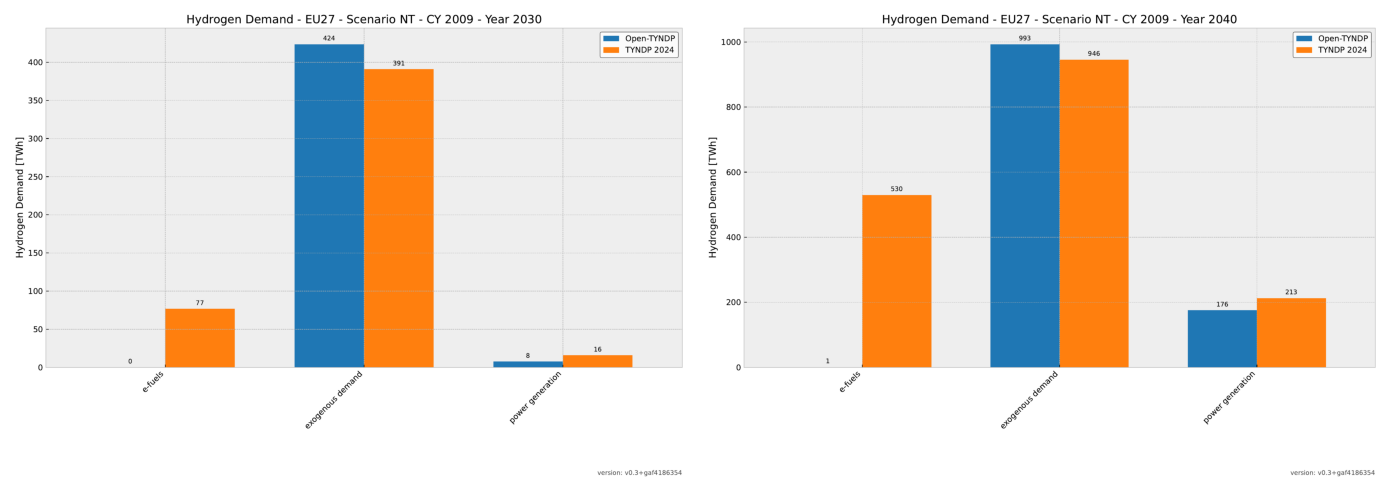
Hydrogen Demand

Since hydrogen demand is primarily defined exogenously, we expect good alignment between model results and TYNDP 2024. However, we observe a large discrepancy for e-fuels production that still needs investigation. The power generation result is determined endogenously and matches the reference values well. Note that hydrogen generation, in contrast, is fully determined by the optimization.

show_benchmarks("benchmark_hydrogen_demand_eu27_cy2009")

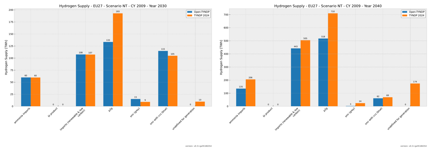
Hydrogen Supply

Hydrogen supply is determined endogenously, and the results are generally convincing, except for power-to-gas (P2G). Since hydrogen demand is exogenous in the NT scenario, the missing P2G production can be explained by the lower hydrogen demand for e-fuels. Additionally, the ‘undefined for generation’ category still needs clarification.

show_benchmarks("benchmark_hydrogen_supply_eu27_cy2009")

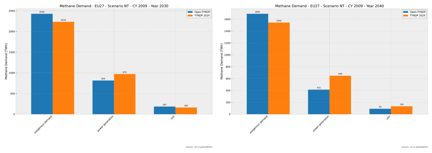
Methane Demand

Methane demand includes both exogenous and endogenous consumption for power generation and steam methane reforming (SMR). The exogenous consumption perfectly reproduces the Supply Tool values. However, alignment with the values reported in the TYNDP 2024 documentation is not yet achieved.

show_benchmarks("benchmark_methane_demand_eu27_cy2009")

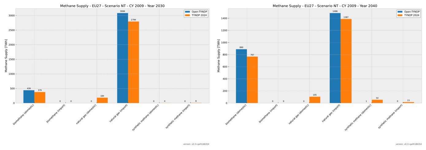
Methane Supply

While the current Open-TYNDP implementation supplies all required methane, it cannot yet accurately reproduce domestic production and imports across all carriers. Natural gas imports include non-EU27 imports, explaining the higher values. The same applies to biomethane.

show_benchmarks("benchmark_methane_supply_eu27_cy2009")

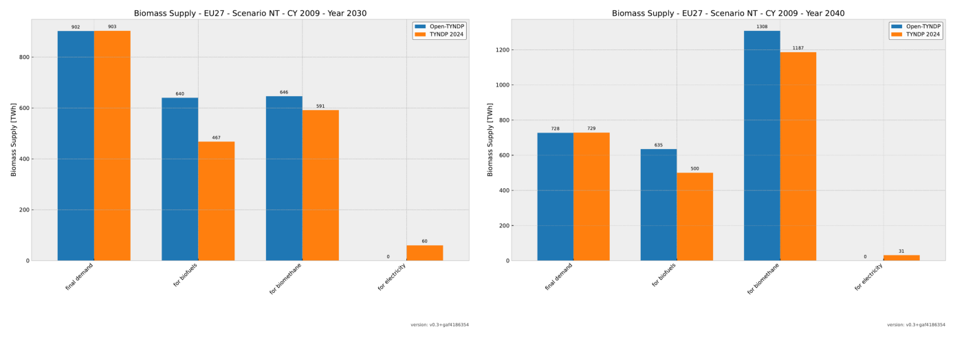
Biomass Supply

The biomass supply correctly reproduces the distribution across different usage categories. However, we observe an overshoot for both biofuels and biomethane. This can be explained by a scope issue, as non-EU27 countries are included in the Open-TYNDP values.

show_benchmarks("benchmark_biomass_supply_eu27_cy2009")

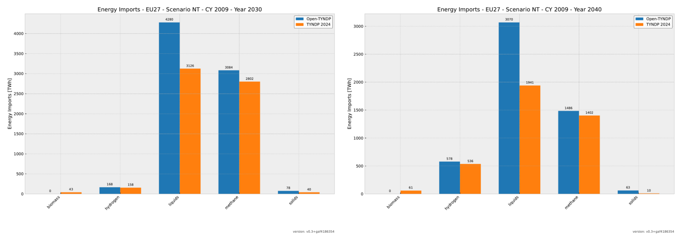
Energy Imports

Energy imports include hydrogen, methane, liquids, and solids. Currently, the model cannot directly import solid biomass. Open-TYNDP values are overestimated because non-EU27 countries contribute to the totals for liquids, methane, and solids. Furthermore, domestic production is not yet removed from the benchmarked values before comparison with TYNDP 2024.

show_benchmarks("benchmark_energy_imports_eu27_cy2009")

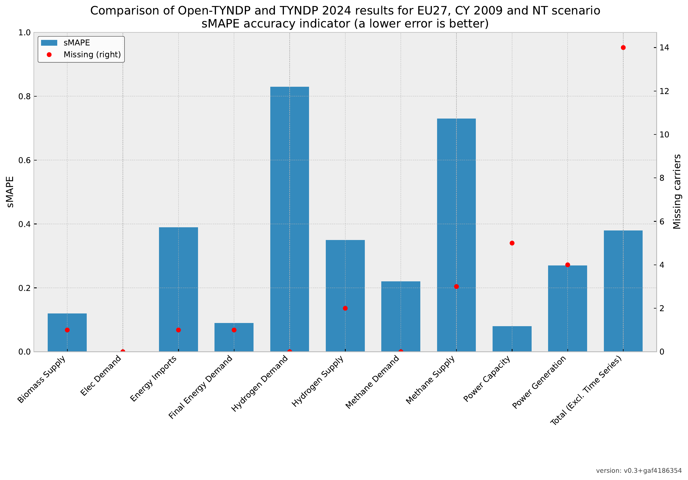
Overview

Finally, let’s examine an overview of the Symmetric Mean Absolute Percentage Error (sMAPE) across all carriers. As a reminder, sMAPE measures the absolute magnitude of deviations while avoiding cancellation between positive and negative errors. This provides a high-level view of error magnitudes across all benchmarks, carriers, and planning horizons.

Note that several features have been significantly improved since we introduced this framework. However, there remains room for further improvement.

It’s important to note that the benchmarking framework is strict regarding missing information. Specifically, sMAPE assigns a large error for missing carriers, which can distort the overall results. This underlines the need for a multi-criteria approach. However, for this assessment, we focus primarily on the sMAPE metric.

display(
    convert_from_path(
        Path("data/results-1H-20251129/validation/kpis_eu27_s_all___all_years.pdf")
    )[0]
)

3. Modify assumptions

A key capability when working with any energy system model is the ability to adjust input assumptions and observe how results respond. This is especially important for TYNDP models, where assumptions evolve over time and multiple configurations need testing.

In Open-TYNDP, there are several straightforward ways to modify assumptions and explore scenarios:

• Input data: Update relevant files in the data folder

• Custom assumptions: Override cost and technology parameters via custom_cost.csv

• Adjustments: Make targeted changes to specific components through configuration files

• Custom constraints: Add or modify constraints directly in the optimization script

Let’s explore each method in detail.

Method 1: Modifying Input Data

The most direct method to modify the model is by editing the input data files. We’ve already retrieved a prebuilt version of the open-tyndp GitHub repository into our working directory dated to the 29th of November 2025.

Navigate to the data directory in the open-tyndp-20251129 repository and locate the tyndp_2024_bundle folder:

from scripts._helpers import display_tree

target_directory = "data/open-tyndp-20251129/data/tyndp_2024_bundle"
print("data")
display_tree(target_directory, max_depth=1)

data
└── tyndp_2024_bundle/
    ├── Demand Profiles/
    ├── EV Modelling Inputs/
    ├── Hybrid Heat Pump Modelling Inputs/
    ├── Hydro Inflows/
    ├── Hydrogen/
    ├── Investment Datasets/
    ├── Line data/
    ├── Nodes/
    ├── Offshore hubs/
    ├── PECD/
    ├── PEMMDB2/
    ├── Supply Tool/
    ├── TYNDP-2024-Scenarios-Package/
    └── TYNDP-2024-Visualisation-Platform/

You can browse and replace any input files with your own data, provided they follow the same format and structure as the original files.

Method 2: Custom Assumptions

To override specific assumptions—such as capital costs, marginal costs, or technical parameters for particular technologies—use a long-format CSV file called custom_cost.csv in the data folder.

Open custom_cost.csv to see example entries that illustrate the required structure:

custom_cost = pd.read_csv("data/open-tyndp-20251129/data/custom_costs.csv")
custom_cost

	planning_horizon	technology	parameter	value	unit	source	further description
0	all	solar	marginal_cost	0.010	EUR/MWh	Default value to prevent mathematical degenera...	NaN
1	all	onwind	marginal_cost	0.015	EUR/MWh	Default value to prevent mathematical degenera...	NaN
2	all	offwind	marginal_cost	0.015	EUR/MWh	Default value to prevent mathematical degenera...	NaN
3	all	hydro	marginal_cost	0.000	EUR/MWh	Default value to prevent mathematical degenera...	NaN
4	all	H2	marginal_cost	0.000	EUR/MWh	Default value to prevent mathematical degenera...	NaN
5	all	electrolysis	marginal_cost	0.000	EUR/MWh	Default value to prevent mathematical degenera...	NaN
6	all	fuel cell	marginal_cost	0.000	EUR/MWh	Default value to prevent mathematical degenera...	NaN
7	all	battery	marginal_cost	0.000	EUR/MWh	Default value to prevent mathematical degenera...	NaN
8	all	battery inverter	marginal_cost	0.000	EUR/MWh	Default value to prevent mathematical degenera...	NaN
9	all	home battery storage	marginal_cost	0.000	EUR/MWh	Default value to prevent mathematical degenera...	NaN
10	all	water tank charger	marginal_cost	0.030	EUR/MWh	Default value to prevent mathematical degenera...	NaN
11	all	central water pit charger	marginal_cost	0.025	EUR/MWh	Default value to prevent mathematical degenera...	NaN

To add your own custom assumptions, insert a new row in this CSV file. At minimum, specify the planning_horizon, technology, parameter, value, and unit for each entry. As shown above, you can also use the all keyword to override a value for all technologies and/or all planning horizons simultaneously.

These custom entries are automatically applied when you run the Open-TYNDP workflow.

Method 3: Adjustments

The third method involves making targeted changes to specific technologies or components directly in the model configuration.

These are called adjustments, and you define them in the scenario configuration file.

Here’s an example from the default configuration file:

def display_code_lines(filename, language, start, end):
    with open(filename) as f:
        lines = f.readlines()
    return Code("".join(lines[start - 1 : end]), language=language)

display_code_lines(
    "data/open-tyndp-20251129/config/config.default.yaml", "yaml", 1066, 1075
)

# docs in https://pypsa-eur.readthedocs.io/en/latest/configuration.html#adjustments
adjustments:
  electricity: false
  sector:
    factor:
      Link:
        electricity distribution grid:
          capital_cost: 1.0
    absolute: false

As shown, you can specify either a scaling factor or an absolute value for any combination of:

• Component type (e.g., Generator, Link, Load)

• Carrier (i.e., technology type)

• Attribute (e.g., marginal_cost, efficiency, p_nom)

To apply manual adjustments to a scenario you’re modeling, add an adjustments section to your scenarios.tyndp.yaml file.

Let’s examine the structure of that file:

display_code_lines(
    "data/open-tyndp-20251129/config/scenarios.tyndp.yaml", "yaml", 1, 150
)

# SPDX-FileCopyrightText: Contributors to Open-TYNDP <https://github.com/open-energy-transition/open-tyndp>
#
# SPDX-License-Identifier: MIT

NT:
  tyndp_scenario: NT
  sector:
    h2_zones_tyndp: false
    co2_sequestration_potential:
      # Values from TYNDP 2024 Supply Tool
      2030: 47
      2035: 167
      2040: 344

NT-52SEG-20251129:
  tyndp_scenario: NT
  sector:
    h2_zones_tyndp: false
    co2_sequestration_potential:
      # Values from TYNDP 2024 Supply Tool
      2030: 47
      2035: 167
      2040: 344
  clustering:
    temporal:
      resolution_sector: 52SEG
  solving:
    solver:
      name: highs
      options: highs-default
    runtime: 12h #runtime in humanfriendly style https://humanfriendly.readthedocs.io/en/latest/

DE:
  tyndp_scenario: DE
  electricity:
    extendable_carriers:
      Generator:
      - onwind
      - solar-pv-utility
      - solar-pv-rooftop
      - offwind-ac-fb-r
      - offwind-ac-fl-r
      - offwind-dc-fb-r
      - offwind-dc-fl-r
      - offwind-dc-fb-oh
      - offwind-dc-fl-oh
      - offwind-h2-fb-oh
      - offwind-h2-fl-oh
      - OCGT
      - CCGT
  sector:
    h2_zones_tyndp: true
    force_biomass_potential: false
    force_biogas_potential: false
    land_transport_ice_share:  # TODO Improve TYNDP 2024 approximations
      2030: 0.96
      2035: 0.7  # interpolation
      2040: 0.44
      2045: 0.3  # interpolation
      2050: 0.16
    co2_sequestration_potential:
      # Values from TYNDP 2024 Supply Tool
      2030: 60
      2035: 90
      2040: 120
      2045: 135
      2050: 150

GA:
  tyndp_scenario: GA
  electricity:
    extendable_carriers:
      Generator:
      - onwind
      - solar-pv-utility
      - solar-pv-rooftop
      - offwind-ac-fb-r
      - offwind-ac-fl-r
      - offwind-dc-fb-r
      - offwind-dc-fl-r
      - offwind-dc-fb-oh
      - offwind-dc-fl-oh
      - offwind-h2-fb-oh
      - offwind-h2-fl-oh
      - OCGT
      - CCGT
  sector:
    h2_zones_tyndp: true
    force_biomass_potential: false
    force_biogas_potential: false
    land_transport_ice_share:  # TODO Improve TYNDP 2024 approximations
      2030: 0.96
      2035: 0.73  # interpolation
      2040: 0.50
      2045: 0.34  # interpolation
      2050: 0.17
    co2_sequestration_potential:
      # Values from TYNDP 2024 Supply
      2030: 48
      2035: 167
      2040: 344
      2045: 398
      2050: 400

Method 4: Custom Constraints

You may also want to add custom constraints to the model. Since we haven’t covered PyPSA constraints in detail yet, we won’t dive deep here—we’ll cover them comprehensively in a future workshop. For now, it’s useful to know where you would add a custom constraint that isn’t already represented through existing component parameters. For more information, see the PyPSA documentation on custom constraints.

Note: Many constraints are already built into PyPSA. For example, to add an upper limit on the expansion capacity of a Link, you can simply use the p_nom_max attribute. PyPSA automatically translates this into a binding upper-limit constraint during optimization.

For custom constraints that go beyond existing parameters, you can insert your own code directly into the model. This flexibility is one of the key advantages of working with an open-source framework.

Navigate to the scripts directory of the open-tyndp-20251129 repository and open the solve_network.py script:

display_code_lines(
    "data/open-tyndp-20251129/scripts/solve_network.py", "Python", 1268, 1361
)

def extra_functionality(
    n: pypsa.Network,
    snapshots: pd.DatetimeIndex,
    planning_horizons: str | None = None,
    offshore_zone_trajectories_fn: str | None = None,
    renewable_carriers_tyndp: list[str] = [],
) -> None:
    """
    Add custom constraints and functionality.

    Parameters
    ----------
    n : pypsa.Network
        The PyPSA network instance with config and params attributes
    snapshots : pd.DatetimeIndex
        Simulation timesteps
    planning_horizons : str, optional
        The current planning horizon year or None in perfect foresight
    offshore_zone_trajectories_fn: str, optional
        Path to the file containing the offshore zone potentials trajectories
    renewable_carriers_tyndp : list[str], optional
        List of TYNDP renewable carriers

    Collects supplementary constraints which will be passed to
    ``pypsa.optimization.optimize``.

    If you want to enforce additional custom constraints, this is a good
    location to add them. The arguments ``opts`` and
    ``snakemake.config`` are expected to be attached to the network.
    """
    config = n.config
    constraints = config["solving"].get("constraints", {})
    if constraints["BAU"] and n.generators.p_nom_extendable.any():
        add_BAU_constraints(n, config)
    if constraints["SAFE"] and n.generators.p_nom_extendable.any():
        add_SAFE_constraints(n, config)
    if constraints["CCL"] and n.generators.p_nom_extendable.any():
        add_CCL_constraints(n, config, planning_horizons)

    reserve = config["electricity"].get("operational_reserve", {})
    if reserve.get("activate"):
        add_operational_reserve_margin(n, snapshots, config)

    if EQ_o := constraints["EQ"]:
        add_EQ_constraints(n, EQ_o.replace("EQ", ""))

    if {"solar-hsat", "solar"}.issubset(
        config["electricity"]["renewable_carriers"]
    ) and {"solar-hsat", "solar"}.issubset(
        config["electricity"]["extendable_carriers"]["Generator"]
    ):
        add_solar_potential_constraints(n, config)

    if n.config.get("sector", {}).get("tes", False):
        if n.buses.index.str.contains(
            r"urban central heat|urban decentral heat|rural heat",
            case=False,
            na=False,
        ).any():
            add_TES_energy_to_power_ratio_constraints(n)
            add_TES_charger_ratio_constraints(n)

    add_battery_constraints(n)
    add_lossy_bidirectional_link_constraints(n)
    add_pipe_retrofit_constraint(n)
    if n._multi_invest:
        add_carbon_constraint(n, snapshots)
        add_carbon_budget_constraint(n, snapshots)
        add_retrofit_gas_boiler_constraint(n, snapshots)
    else:
        add_co2_atmosphere_constraint(n, snapshots)

    if config["sector"]["enhanced_geothermal"]["enable"]:
        add_flexible_egs_constraint(n)

    if config["sector"]["imports"]["enable"]:
        add_import_limit_constraint(n, snapshots)

    if config["sector"]["offshore_hubs_tyndp"]["enable"]:
        add_offshore_hubs_constraint(
            n,
            int(planning_horizons),
            offshore_zone_trajectories_fn,
            renewable_carriers_tyndp,
        )

    if n.params.custom_extra_functionality:
        source_path = n.params.custom_extra_functionality
        assert os.path.exists(source_path), f"{source_path} does not exist"
        sys.path.append(os.path.dirname(source_path))
        module_name = os.path.splitext(os.path.basename(source_path))[0]
        module = importlib.import_module(module_name)
        custom_extra_functionality = getattr(module, module_name)
        custom_extra_functionality(n, snapshots, snakemake)  # pylint: disable=E0601

In solve_network.py, you’ll find a function called extra_functionality. This is where additional custom constraints are added to the optimization model before solving.

For instance, Open-TYNDP includes a custom constraint for offshore hubs by calling the nested function add_offshore_hubs_constraint. This constraint limits the expansion of DC and H2 wind farms at the same location and enforces maximum potential per zone according to zone trajectories.

You can add your own constraints in the same location. Browse the existing constraint implementations to understand the structure and coding style.

We’ll cover PyPSA constraint mechanics in depth in a future workshop.

Task 1: Apply Manual Adjustments

Open data/open-tyndp-20251129/config/scenarios.tyndp.yaml and modify the existing NT-52SEG-20251129 scenario by adding the following manual adjustments:

• Increase the marginal_cost of all H2 imports by a factor of 1.5 (2030) and 1.3 (2040). The supply of imported H2 is included as a Generator component with the carrier name import H2.

• Change the efficiency of H2 Electrolysis to 78% for both 2030 and 2040. H2 Electrolysis is added as a Link component.

• Remove the initial capacity (p_nom and p_nom_min) of all solar-pv-utility generators for 2030.

Then rerun the model and explore the results in PyPSA-Explorer.

Hint: If you need a reminder on running the Snakemake workflow, refer to the notebook from our last workshop.

Hint II: Always start with a dry run first (add -n to your Snakemake command).

Hint III: As we only want to solve the model without post-processing, we can call the rule solve_sector_networks instead of the all rule.

Hint IV: Make sure that the scenario that you want to run is specifying a solver that you can use. You can change the solver to Highs (an open-source solver) by changing the following configuration: solving:solver.

To run the workflow, we first need to install and activate the open-tyndp environment.

The recommended approach for PyPSA models is to use the pixi environment manager, which handles all dependencies automatically.

Note

We are currently working on a robust setup for all operating systems and will focus on this topic specifically in our next workshop.

If you prefer to use conda to install the open-tyndp environment locally, refer to our legacy installation documentation.

To install pixi locally on your operating system, follow the steps in the official pixi installation documentation.

For execution on Google Colab, install the Linux version of pixi in the runtime:

!wget -qO- https://pixi.sh/install.sh | sh

In the Google Colab terminal, you might need to execute:

exec bash -l

for the changes to take effect if pixi is not recognized.

# Uncomment the next line for running this notebook on Colab
# !wget -qO- https://pixi.sh/install.sh | sh

Next, open a terminal window. Navigate to the open-tyndp-20251129 repository before launching the workflow:

cd data/open-tyndp-20251129

Once you’re in the open-tyndp-20251129 repository, activate the environment with pixi. This drops you into a shell where you can run the workflow:

pixi shell -e open-tyndp

Solutions

Task 1: Apply Manual Adjustments

Add the following adjustments section to the NT-52SEG-20251129 scenario configuration in scenarios.tyndp.yaml:

adjustments:
  sector:
    factor:
      Generator:
        import H2:
          marginal_cost:
            2030: 1.5
            2040: 1.3
        solar-pv-utility:
          p_nom:
            2030: 0.0
    absolute:
      Link:
        H2 Electrolysis:
          efficiency:
            2030: 0.78
            2040: 0.78

In a terminal window, we start with a dry run to preview which rules will execute:

snakemake --call solve_sector_networks --configfile config/config.tyndp.yaml -n

After adding the adjustments to scenarios.tyndp.yaml, we can run the Open-TYNDP workflow using Snakemake with the standard config.tyndp.yaml configuration.

The dry run shows that, because this scenario was run previously without the adjustments, Snakemake will only re-execute the rules affected by your manual changes.

Now run the workflow for real:

snakemake --call solve_sector_networks --configfile config/config.tyndp.yaml

Finally, let’s launch PyPSA-Explorer again to inspect the results of our modified scenario.

First, we load the new outputs into our networks dictionary:

# Load networks directly into dictionary for PyPSA-Explorer
base_path = "data/open-tyndp-20251129/results/tyndp/NT-52SEG-20251129/networks/"
networks.update(
    {
        "NT 2030 new": import_network(base_path + "base_s_all___2030.nc"),
        "NT 2040 new": import_network(base_path + "base_s_all___2040.nc"),
    }
)

# set a new port for the updated dashboard
port = 8051

WARNING:pypsa.network.io:Importing network from PyPSA version v1.0.4 while current version is v1.0.5. Read the release notes at `https://go.pypsa.org/release-notes` to prepare your network for import.

INFO:pypsa.network.io:Imported network 'PyPSA-Eur (tyndp)' has buses, carriers, generators, global_constraints, links, loads, shapes, storage_units, stores, sub_networks

WARNING:pypsa.network.io:Importing network from PyPSA version v1.0.4 while current version is v1.0.5. Read the release notes at `https://go.pypsa.org/release-notes` to prepare your network for import.

INFO:pypsa.network.io:Imported network 'PyPSA-Eur (tyndp)' has buses, carriers, generators, global_constraints, links, loads, shapes, storage_units, stores, sub_networks

# Terminal method recommended
USE_TERMINAL = True  # Change to False if you want to launch inline display

if not IN_COLAB and not USE_TERMINAL:
    # Local Jupyter: Inline display
    app = create_app(networks)
    app.run(jupyter_mode="tab", port=port, debug=False)

if IN_COLAB:
    run_pypsa_explorer_in_colab(networks, port)

Notebook clean up

# Only clean up data when running in CI environment
if os.getenv("CI"):
    rm_dir = "data/open-tyndp-20251129"
    print(
        f"CI environment detected. Cleaning up notebook data by removing '{rm_dir}' and '{rm_dir}.zip'."
    )
    shutil.rmtree(rm_dir, ignore_errors=True)
    Path(f"{rm_dir}.zip").unlink(missing_ok=True)
else:
    print("Skipping cleanup (not in CI environment).")

CI environment detected. Cleaning up notebook data by removing 'data/open-tyndp-20251129' and 'data/open-tyndp-20251129.zip'.