Workshop 2: Introduction to Snakemake, new features update & benchmarking#
Note
At the end of this notebook, you will be able to:
Describe key concepts of workflow tools such as Snakemake
Navigate the Open-TYNDP folder structure
Execute all or specific rules within the Open-TYNDP Snakemake workflow
Explain the new features added to Open-TYNDP v0.3
Use the benchmarking framework
Note
If you have not yet set up Python on your computer, you can execute this tutorial in your browser via Google Colab. Click on the rocket in the top right corner and launch “Colab”. If that doesn’t work download the .ipynb file and import it in Google Colab.
Then install the following packages by executing the following command in a Jupyter cell at the top of the notebook.
!pip install pypsa pandas geopandas xarray matplotlib seaborn cartopy snakemake graphviz snakemake-storage-plugin-http pdf2image atlite fiona powerplantmatching folium mapclassify
!apt-get install poppler-utils
# uncomment for running this notebook on Colab
# !pip install pypsa pandas geopandas xarray matplotlib seaborn cartopy snakemake graphviz snakemake-storage-plugin-http pdf2image atlite fiona powerplantmatching folium mapclassify
# !apt-get install poppler-utils
import os
import shutil
import zipfile
from datetime import datetime
from pathlib import Path
from urllib.request import urlretrieve

import cartopy.crs as ccrs
import matplotlib.pyplot as plt
import numpy as np
import pandas as pd
import pypsa
import seaborn as sns
import warnings
from IPython.display import Code, SVG, Image, IFrame, display
from matplotlib.ticker import MultipleLocator
from pdf2image import convert_from_path
from pypsa.plot.maps.static import (
    add_legend_circles,
    add_legend_lines,
    add_legend_patches,
)

pypsa.options.params.statistics.round = 3
pypsa.options.params.statistics.drop_zero = True
pypsa.options.params.statistics.nice_names = False
plt.rcParams["figure.figsize"] = [14, 7]
def unzip_with_timestamps(zip_path, extract_to, keep_zip=True):
    """Unzip a file while preserving original file timestamps."""
    with zipfile.ZipFile(zip_path, "r") as zip_ref:
        for member in zip_ref.infolist():
            # Extract the file
            zip_ref.extract(member, extract_to)

            # Get the extracted file path
            extracted_path = os.path.join(extract_to, member.filename)

            # Get the modification time from the zip file
            date_time = datetime(*member.date_time)
            timestamp = date_time.timestamp()

            # Set both access and modification times
            os.utime(extracted_path, (timestamp, timestamp))
    if not keep_zip:
        os.remove(zip_path)
urls = {
    "data/data_raw.csv": "https://storage.googleapis.com/open-tyndp-data-store/workshop-02/data_raw.csv",
    "data/open-tyndp-20251016.zip": "https://storage.googleapis.com/open-tyndp-data-store/workshop-02/open-tyndp-20251016.zip",
    "data/network_NT_presolve_highres_2030.nc": "https://storage.googleapis.com/open-tyndp-data-store/workshop-02/network_NT_presolve_highres_2030.nc",
    "Snakefile": "https://raw.githubusercontent.com/open-energy-transition/open-tyndp-workshops/792b8474ab5096e5ab8db2822af4fcd9fe659eb6/open-tyndp-workshops/Snakefile",
    "scripts/build_data.py": "https://raw.githubusercontent.com/open-energy-transition/open-tyndp-workshops/792b8474ab5096e5ab8db2822af4fcd9fe659eb6/open-tyndp-workshops/scripts/build_data.py",
    "scripts/prepare_network.py": "https://raw.githubusercontent.com/open-energy-transition/open-tyndp-workshops/792b8474ab5096e5ab8db2822af4fcd9fe659eb6/open-tyndp-workshops/scripts/prepare_network.py",
    "scripts/filter_dag.py": "https://raw.githubusercontent.com/open-energy-transition/open-tyndp-workshops/792b8474ab5096e5ab8db2822af4fcd9fe659eb6/open-tyndp-workshops/scripts/filter_dag.py",
}

os.makedirs("data", exist_ok=True)
os.makedirs("scripts", exist_ok=True)
for name, url in urls.items():
    if os.path.exists(name):
        print(f"File {name} already exists. Skipping download.")
    else:
        print(f"Retrieving {name} from storage.")
        urlretrieve(url, name)
        print(f"File available in {name}.")

to_dir = "data/open-tyndp-20251016"
if not os.path.exists(to_dir):
    print(f"Unzipping data/open-tyndp-20251016.zip.")
    unzip_with_timestamps("data/open-tyndp-20251016.zip", "data/open-tyndp-20251016")
print(f"Open-TYNDP available in '{to_dir}'.")

print("Done")
Retrieving data/data_raw.csv from storage.
File available in data/data_raw.csv.
Retrieving data/open-tyndp-20251016.zip from storage.
File available in data/open-tyndp-20251016.zip.
Retrieving data/network_NT_presolve_highres_2030.nc from storage.
File available in data/network_NT_presolve_highres_2030.nc.
File Snakefile already exists. Skipping download.
File scripts/build_data.py already exists. Skipping download.
File scripts/prepare_network.py already exists. Skipping download.
File scripts/filter_dag.py already exists. Skipping download.
Unzipping data/open-tyndp-20251016.zip.
Open-TYNDP available in 'data/open-tyndp-20251016'.
Done
The Snakemake tool#
The Snakemake workflow management system is a tool to create reproducible and scalable data analyses.
Workflows are described via a human readable, Python based language. They can be seamlessly scaled to server, cluster, grid, and cloud environments, without the need to modify the workflow definition.
Snakemake follows the GNU Make paradigm: workflows are defined in terms of so-called rules that specify how to create a set of output files from a set of input files. Dependencies between the rules are determined automatically, creating a DAG (directed acyclic graph) of jobs that can be automatically parallelized.
Note
Documentation for this package is available at https://snakemake.readthedocs.io/. You can also check out a slide deck Snakemake Tutorial by Johannes Köster (2024).
Mölder, F., Jablonski, K.P., Letcher, B., Hall, M.B., Tomkins-Tinch, C.H., Sochat, V., Forster, J., Lee, S., Twardziok, S.O., Kanitz, A., Wilm, A., Holtgrewe, M., Rahmann, S., Nahnsen, S., Köster, J., 2021. Sustainable data analysis with Snakemake. F1000Res 10, 33.
A minimal Snakemake example#
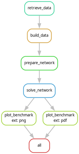
To check out how this looks in practice, we’ve prepared a minimal Snakemake example workflow that processes some data. The minimal workflow consists of the following rules:
retrieve_databuild_dataprepare_networksolve_networkplot_benchmarkall
These rules are illustrative and mimic the Open-TYNDP structure and nomenclature.
We have already loaded the raw data file used in this minimal example into our working directory.
As you can see, the plot_benchmark rule will be called twice with two different filename extensions. For this, we are taking advantage of the concept of wildcards (ext). Snakemake will automatically resolve the wildcards using the dependency graph. In this case, the all rule takes as input both a png and a pdf figure which propagates back throughout the workflow.
The Snakefile and rules#
The rules need to be defined in a so-called Snakefile that sits in your current working directory. For our minimal example the Snakefile looks like this:
Code(filename="Snakefile", language="Python")
# SPDX-FileCopyrightText: Open Energy Transition gGmbH
#
# SPDX-License-Identifier: MIT

from pathlib import Path

rule all:
    input:
        "data/benchmark.png",
        "data/benchmark.pdf"

rule retrieve_data:
    output:
        "data/data_raw.csv"
    shell:
        "wget -O {output} https://storage.googleapis.com/open-tyndp-data-store/workshop-02/data_raw.csv"

rule build_data:
    input:
        "data/data_raw.csv"
    output:
        "data/data_filtered.csv"
    script:
        "scripts/build_data.py"

rule prepare_network:
    input:
        "data/data_filtered.csv"
    output:
        "data/base_2030.nc"
    script:
        "scripts/prepare_network.py"

rule solve_network:
    input:
        "data/base_2030.nc"
    output:
        "data/base_2030_solved.nc"
    shell:
        "cp {input} {output}"

rule plot_benchmark:
    input:
        "data/base_2030_solved.nc"
    output:
        "data/benchmark.{ext}"
    run:
        Path(output[0]).touch()
You can check out the scripts under scripts. You will see that they are simplistic and only serve an illustrative purpose.
You can also observe how the plot_benchmark rule is defined to take advantage of the wildcards. This reduces the redundancy in the Snakefile. Wildcards are defined between { } in the rule definition.
Calling a workflow#
You can trigger the workflow by specifying a target file, like data/benchmark.pdf, or any intermediate file:
snakemake -call data/benchmark.pdf
Alternatively, you can also execute the workflow by calling a rule that produces an intermediate file:
snakemake -call build_data
NOTE: You cannot call a rule that includes a wildcard without specifying what the wildcard should be filled with. Otherwise, Snakemake will not know what to propagate back.
Or you can call the common rule all which can be used to execute the entire workflow. It takes the final workflow output as its input and thus requires all previous dependent rules to be run as well:
snakemake -call all
Because we defined the all rule as first in the Snakefile, this rule is assumed to be the default and the following also works:
snakemake -call
A very important feature is the -n flag which executes a dry-run. It is recommended to always first execute a dry-run before the actual execution of a workflow. This simply prints out the DAG of the workflow to investigate without actually executing it.
Let’s try this out and investigate the output:
! snakemake -call -n
SNAKEMAKE
=========
  Date: 2026-07-09 11:59:37
  Workflow ID: ebbda29e-6e36-4c27-977f-d9ee866536b3
  Platform: Linux-6.17.0-1018-azure-x86_64-with-glibc2.39
  Host: runnervm5mmn9
  User: runner
  Snakemake version: 9.23.1
  Python version: 3.13.14 | packaged by conda-forge | (main, Jun 12 2026, 09:50:25) [GCC 14.3.0]
  Command: /home/runner/miniconda3/envs/open-tyndp-workshops/bin/snakemake -call -n
  Snakefile: /home/runner/work/open-tyndp-workshops/open-tyndp-workshops/open-tyndp-workshops/Snakefile
  Base directory: /home/runner/work/open-tyndp-workshops/open-tyndp-workshops/open-tyndp-workshops
  Run directory: /home/runner/work/open-tyndp-workshops/open-tyndp-workshops/open-tyndp-workshops
  Working directory: /home/runner/work/open-tyndp-workshops/open-tyndp-workshops/open-tyndp-workshops
  Config file(s): []
  Config MD5: 99914b932bd37a50b983c5e7c90ae93b

Building DAG of jobs...
Job stats:
job                count
---------------  -------
build_data             1
prepare_network        1
solve_network          1
plot_benchmark         2
all                    1
total                  6


[Thu Jul  9 11:59:38 2026]
rule build_data:
    input: data/data_raw.csv
    output: data/data_filtered.csv
    jobid: 4
    reason: Missing output files: data/data_filtered.csv
    resources: tmpdir=/tmp
[Thu Jul  9 11:59:38 2026]
rule prepare_network:
    input: data/data_filtered.csv
    output: data/base_2030.nc
    jobid: 3
    reason: Missing output files: data/base_2030.nc; Input files updated by another job: data/data_filtered.csv
    resources: tmpdir=/tmp
[Thu Jul  9 11:59:38 2026]
rule solve_network:
    input: data/base_2030.nc
    output: data/base_2030_solved.nc
    jobid: 2
    reason: Missing output files: data/base_2030_solved.nc; Input files updated by another job: data/base_2030.nc
    resources: tmpdir=/tmp
[Thu Jul  9 11:59:38 2026]
rule plot_benchmark:
    input: data/base_2030_solved.nc
    output: data/benchmark.png
    jobid: 1
    reason: Missing output files: data/benchmark.png; Input files updated by another job: data/base_2030_solved.nc
    wildcards: ext=png
    resources: tmpdir=/tmp
[Thu Jul  9 11:59:38 2026]
rule plot_benchmark:
    input: data/base_2030_solved.nc
    output: data/benchmark.pdf
    jobid: 6
    reason: Missing output files: data/benchmark.pdf; Input files updated by another job: data/base_2030_solved.nc
    wildcards: ext=pdf
    resources: tmpdir=/tmp
[Thu Jul  9 11:59:38 2026]
rule all:
    input: data/benchmark.png, data/benchmark.pdf
    jobid: 0
    reason: Input files updated by another job: data/benchmark.pdf, data/benchmark.png
    resources: tmpdir=/tmp
Job stats:
job                count
---------------  -------
build_data             1
prepare_network        1
solve_network          1
plot_benchmark         2
all                    1
total                  6

Reasons:
    (check individual jobs above for details)
    input files updated by another job:
        all, plot_benchmark, prepare_network, solve_network
    output files have to be generated:
        build_data, plot_benchmark, prepare_network, solve_network
1 jobs have missing provenance/metadata so that it in part cannot be used to trigger re-runs.
Rules with missing metadata: retrieve_data
This was a dry-run (flag -n). The order of jobs does not reflect the order of execution.
As you can see, the plot_benchmark rule will be executed twice due to wildcards.
Visualizing the DAG of a workflow#
You can also visualize the DAG of jobs using the --dag flag and the Graphviz dot command. This will not run the workflow but only create the visualization:
! snakemake -call --dag | python scripts/filter_dag.py | dot -Tpng -o dag_minimal.png
# For Windows run instead:
# ! snakemake -call --dag | python scripts\\filter_dag.py | dot -Tpng -o dag_minimal.png
Building DAG of jobs...
Image("dag_minimal.png")
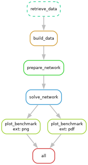
Rules that need to be executed will be presented as plain lines, while those that have already been executed will be presented as dotted lines. An alternative to the DAG is the rulegraph. This graph is typically less crowded as you will only visualize the dependency graph of rules. This representation is leaner than the DAG because rules are not repeated for wildcards.
! snakemake -call all --rulegraph | python scripts/filter_dag.py | dot -Tpng -o rulegraph_minimal.png
# For Windows run instead:
# ! snakemake -call all --rulegraph | python scripts\\filter_dag.py | dot -Tpng -o rulegraph_minimal.png
Building DAG of jobs...
Image("rulegraph_minimal.png")
As you can see, the plot_benchmark rule is only represented once.
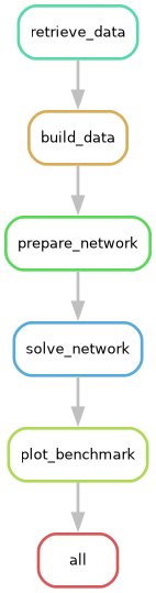
Alternatively, you can also visualize a filegraph, which is similar to the rulegraph but includes some information about the inputs and outputs to each of the rules.
! snakemake -call all --filegraph | python scripts/filter_dag.py | dot -Tsvg -o filegraph_minimal.svg
# For Windows run instead:
# ! snakemake -call all --filegraph | python scripts\\filter_dag.py | dot -Tsvg -o filegraph_minimal.svg
Building DAG of jobs...
SVG("filegraph_minimal.svg")

Task 1: Executing a workflow with Snakemake#
a) For our minimal example, execute a dry-run to produce the intermediate file data/base_2030.nc.
b) Execute the entire workflow and investigate what happens if you try to execute the workflow again.
c) Delete the final output file data/benchmark.pdf and investigate what happens if you try to execute the workflow again.
d) Change a value in the raw input data file data/data_raw.csv and save it again, overwriting the original file. Investigate what happens if you try to execute the workflow again.
Hint: You can also just touch the file by executing Path("data/data_raw.csv").touch(). This will mimic a file edit.
e) (Optional) Open the Snakefile and add a second rule that processes the file data_raw_2.csv using the same script as the build_data rule. Add the output of this new rule as a second input to the prepare_network rule.
# Your solution a)
# Your solution b)
# Your solution c)
# Your solution d)
# Your solution e)
Discover Open-TYNDP file structure#
We have already retrieved a prebuilt version of the open-tyndp GitHub repository into our working directory dated to the 16th of October 2025. This folder contains a run of Open-TYNDP for NT and DE scenarios, with 2030 and 2040 as planning horizons. We removed the atlite cutout from the archive and compressed the archive using zip -r open-tyndp-20251016.zip ..
The open-tyndp-20251016 repository contains the following structure. Directories of particular interest are marked in bold:
benchmarks: will store Snakemake benchmarks (does not exist initially)
config: configurations used in the study
cutouts: will store raw weather data cutouts from atlite (does not exist initially)
data: includes input data that is not produced by any Snakemake rule. Various different input files are retrieved from external storage and stored in this directory
doc: includes all files necessary to build the readthedocs documentation of PyPSA-Eur
envs: includes all the mamba environment specifications to run the workflow
logs: will store log files (does not exist initially)
notebooks: includes all the notebooks used for ad-hoc analysis
report: contains all files necessary to build the report; plots and result files are generated automatically
rules: includes all the Snakemake rules loaded in the Snakefile
resources: will store intermediate results of the workflow which can be picked up again by subsequent rules (does not exist initially)
results: will store the solved PyPSA network data, summary files and output plots (does not exist initially)
scripts: includes all the Python scripts executed by the Snakemake rules to build the model
Task 2: Explore the folder#
a) Can you find the TYNDP specific data input files?
b) Where can you check which scenario and planning horizons were used to generate the current results?
Hint: Search for config.tyndp.yaml.
c) Can you find the hydrogen grid map in the output files for the NT scenario in 2040?
Hint: Search for base_s_all__-h2_network_2040.pdf.
# Your solution a)
# Your solution b)
# Your solution c)
Using Snakemake to launch the Open-TYNDP workflow#
We now need to change our working directory to the Open-TYNDP directory we previously retrieved.
os.chdir("data/open-tyndp-20251016")
Be aware that to run the previous section of this notebook, you will need to restore the default working directory using os.chdir("../../").
Let’s check that we are indeed in the new directory now:
os.getcwd()
'/home/runner/work/open-tyndp-workshops/open-tyndp-workshops/open-tyndp-workshops/data/open-tyndp-20251016'
We can now use Snakemake to call some of the rules to produce outputs with the open-tyndp PyPSA model.
We will use the prepared TYNDP configuration file (config/config.tyndp.yaml) and schedule a dry-run with -n as we only want to investigate the DAG of the workflow:
! snakemake -call --configfile config/config.tyndp.yaml -n
Config file config/config.default.yaml is extended by additional config specified via the command line.
Config file config/plotting.default.yaml is extended by additional config specified via the command line.
Config file config/benchmarking.default.yaml is extended by additional config specified via the command line.
Config file config/config.private.yaml is extended by additional config specified via the command line.
Datafile downloads disabled in config[retrieve] or no internet access.
SNAKEMAKE
=========
  Date: 2026-07-09 11:59:44
  Workflow ID: 1f9d83c3-d0ed-44ec-9907-c22e2b692ecb
  Platform: Linux-6.17.0-1018-azure-x86_64-with-glibc2.39
  Host: runnervm5mmn9
  User: runner
  Snakemake version: 9.23.1
  Python version: 3.13.14 | packaged by conda-forge | (main, Jun 12 2026, 09:50:25) [GCC 14.3.0]
  Command: /home/runner/miniconda3/envs/open-tyndp-workshops/bin/snakemake -call --configfile config/config.tyndp.yaml -n
  Snakefile: /home/runner/work/open-tyndp-workshops/open-tyndp-workshops/open-tyndp-workshops/data/open-tyndp-20251016/Snakefile
  Base directory: /home/runner/work/open-tyndp-workshops/open-tyndp-workshops/open-tyndp-workshops/data/open-tyndp-20251016
  Run directory: /home/runner/work/open-tyndp-workshops/open-tyndp-workshops/open-tyndp-workshops/data/open-tyndp-20251016
  Working directory: /home/runner/work/open-tyndp-workshops/open-tyndp-workshops/open-tyndp-workshops/data/open-tyndp-20251016
  Config file(s): [PosixPath('/home/runner/work/open-tyndp-workshops/open-tyndp-workshops/open-tyndp-workshops/data/open-tyndp-20251016/config/config.tyndp.yaml'), 'config/config.default.yaml', 'config/plotting.default.yaml', 'config/benchmarking.default.yaml', 'config/config.private.yaml']
  Config MD5: e1b8c0df6d43bd15b94893013ba0fb54

Building DAG of jobs...
Nothing to be done (all requested files are present and up to date).
As you can see, there is nothing to be done since all necessary outputs are already present in the files. However, we can still explore the set of rules defined in the Snakefile and the other .smk files. First, we can plot the rule graph, then the full DAG.
The corresponding rule graph to this workflow will look like this:
! snakemake -call --configfile config/config.tyndp.yaml --rulegraph | python ../../scripts/filter_dag.py | dot -Tpng -o rulegraph_open_tyndp.png
# For Windows run instead:
# ! snakemake -call --configfile config/config.tyndp.yaml --rulegraph | python ..\\..\\scripts\\filter_dag.py | dot -Tpng -o rulegraph_open_tyndp.png
Config file config/config.default.yaml is extended by additional config specified via the command line.
Config file config/plotting.default.yaml is extended by additional config specified via the command line.
Config file config/benchmarking.default.yaml is extended by additional config specified via the command line.
Config file config/config.private.yaml is extended by additional config specified via the command line.
Building DAG of jobs...
Image("rulegraph_open_tyndp.png")
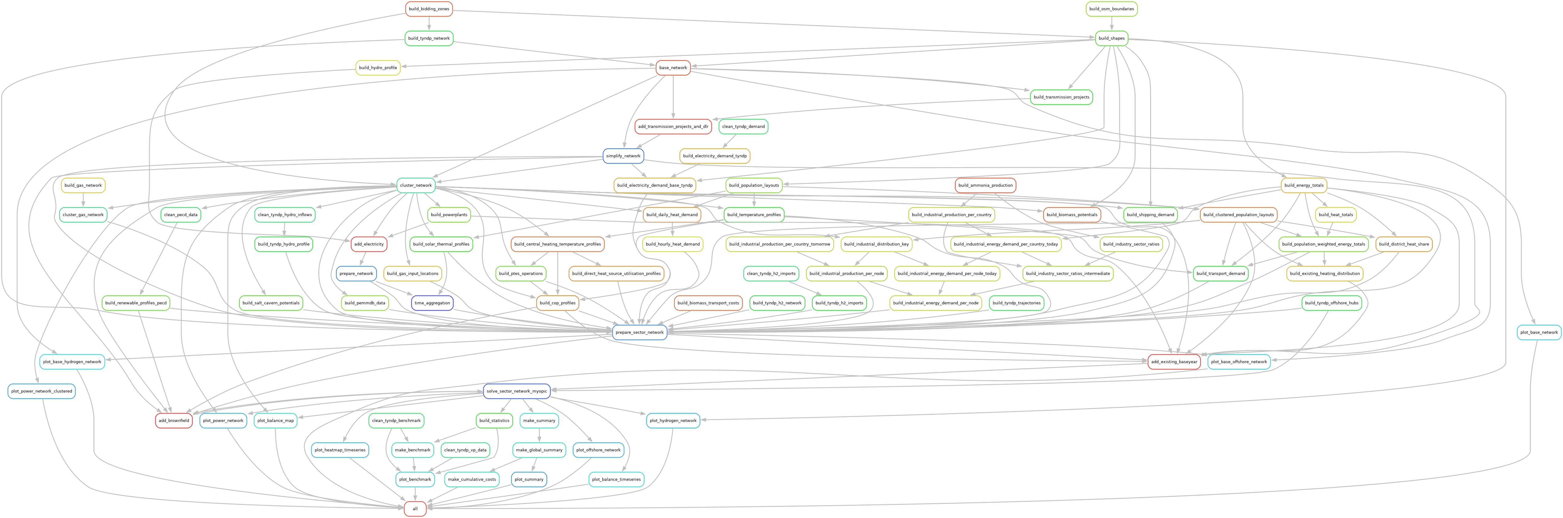
The corresponding DAG to this workflow will look like this:
! snakemake -call --configfile config/config.tyndp.yaml --dag | python ../../scripts/filter_dag.py | dot -Tpng -o dag_open_tyndp.png
# For Windows run instead:
# ! snakemake -call --configfile config/config.tyndp.yaml --dag | python ..\\..\\scripts\\filter_dag.py | dot -Tpng -o dag_open_tyndp.png
Config file config/config.default.yaml is extended by additional config specified via the command line.
Config file config/plotting.default.yaml is extended by additional config specified via the command line.
Config file config/benchmarking.default.yaml is extended by additional config specified via the command line.
Config file config/config.private.yaml is extended by additional config specified via the command line.
Building DAG of jobs...
Image("dag_open_tyndp.png")
As you can see, this workflow is much more complex than our minimal example from the beginning. Since we already executed the entire workflow for this demonstration, all the rules are presented as dotted lines in the DAG.
You will also notice that the DAG is much larger than the rule graph. This is because Open-TYNDP leverages wildcards quite extensively to generalize rule definitions and to parallelize tasks.
Nevertheless, the general idea remains the same. We retrieve data which we consequently process, then we prepare the model network and we solve it before we postprocess the results (summary, plotting, benchmarks).
Triggering a workflow run on Open-TYNDP#
Let’s simulate a completed optimization by updating the timestamp of the solved network file (base_s_all___2040.nc), which is saved as the final step of the optimization process.
Path("results/tyndp/NT/networks/base_s_all___2040.nc").touch()
We can now see that Snakemake triggers all the rules that depend on the solved network. In this case, these are all the postprocessing rules.
! snakemake -call --configfile config/config.tyndp.yaml -n
Config file config/config.default.yaml is extended by additional config specified via the command line.
Config file config/plotting.default.yaml is extended by additional config specified via the command line.
Config file config/benchmarking.default.yaml is extended by additional config specified via the command line.
Config file config/config.private.yaml is extended by additional config specified via the command line.
Datafile downloads disabled in config[retrieve] or no internet access.
SNAKEMAKE
=========
  Date: 2026-07-09 11:59:59
  Workflow ID: 437c6638-9b05-4ec9-8c46-4c0eec9e4549
  Platform: Linux-6.17.0-1018-azure-x86_64-with-glibc2.39
  Host: runnervm5mmn9
  User: runner
  Snakemake version: 9.23.1
  Python version: 3.13.14 | packaged by conda-forge | (main, Jun 12 2026, 09:50:25) [GCC 14.3.0]
  Command: /home/runner/miniconda3/envs/open-tyndp-workshops/bin/snakemake -call --configfile config/config.tyndp.yaml -n
  Snakefile: /home/runner/work/open-tyndp-workshops/open-tyndp-workshops/open-tyndp-workshops/data/open-tyndp-20251016/Snakefile
  Base directory: /home/runner/work/open-tyndp-workshops/open-tyndp-workshops/open-tyndp-workshops/data/open-tyndp-20251016
  Run directory: /home/runner/work/open-tyndp-workshops/open-tyndp-workshops/open-tyndp-workshops/data/open-tyndp-20251016
  Working directory: /home/runner/work/open-tyndp-workshops/open-tyndp-workshops/open-tyndp-workshops/data/open-tyndp-20251016
  Config file(s): [PosixPath('/home/runner/work/open-tyndp-workshops/open-tyndp-workshops/open-tyndp-workshops/data/open-tyndp-20251016/config/config.tyndp.yaml'), 'config/config.default.yaml', 'config/plotting.default.yaml', 'config/benchmarking.default.yaml', 'config/config.private.yaml']
  Config MD5: e1b8c0df6d43bd15b94893013ba0fb54

Building DAG of jobs...
Job stats:
job                        count
-----------------------  -------
build_statistics               1
make_summary                   1
plot_balance_map               6
plot_balance_timeseries        1
plot_heatmap_timeseries        1
plot_hydrogen_network          1
plot_offshore_network          2
plot_power_network             1
make_benchmark                 1
make_global_summary            1
make_cumulative_costs          1
plot_benchmark                 1
plot_summary                   1
all                            1
total                         20


[Thu Jul  9 12:00:01 2026]
rule make_summary:
    input: results/tyndp/NT/networks/base_s_all___2040.nc
    output: results/tyndp/NT/csvs/individual/nodal_costs_s_all___2040.csv, results/tyndp/NT/csvs/individual/nodal_capacities_s_all___2040.csv, results/tyndp/NT/csvs/individual/nodal_capacity_factors_s_all___2040.csv, results/tyndp/NT/csvs/individual/capacity_factors_s_all___2040.csv, results/tyndp/NT/csvs/individual/costs_s_all___2040.csv, results/tyndp/NT/csvs/individual/capacities_s_all___2040.csv, results/tyndp/NT/csvs/individual/curtailment_s_all___2040.csv, results/tyndp/NT/csvs/individual/energy_s_all___2040.csv, results/tyndp/NT/csvs/individual/energy_balance_s_all___2040.csv, results/tyndp/NT/csvs/individual/nodal_energy_balance_s_all___2040.csv, results/tyndp/NT/csvs/individual/prices_s_all___2040.csv, results/tyndp/NT/csvs/individual/weighted_prices_s_all___2040.csv, results/tyndp/NT/csvs/individual/market_values_s_all___2040.csv, results/tyndp/NT/csvs/individual/metrics_s_all___2040.csv
    log: results/tyndp/NT/logs/make_summary_s_all___2040.log
    jobid: 240
    benchmark: results/tyndp/NT/benchmarks/make_summary_s_all___2040
    reason: Updated input files: results/tyndp/NT/networks/base_s_all___2040.nc
    wildcards: run=NT, clusters=all, opts=, sector_opts=, planning_horizons=2040
    resources: tmpdir=/tmp, mem_mb=8000, mem=8 GB, mem_mib=7630
[Thu Jul  9 12:00:01 2026]
rule plot_offshore_network:
    input: results/tyndp/NT/networks/base_s_all___2040.nc
    output: results/tyndp/NT/maps/base_s_all___2040-offshore_network_DC_OH.pdf
    log: results/tyndp/NT/logs/plot_offshore_network_all___2040_DC_OH.log
    jobid: 212
    benchmark: benchmarks/tyndp/NT/plot_offshore_network_all___2040_DC_OH
    reason: Updated input files: results/tyndp/NT/networks/base_s_all___2040.nc
    wildcards: run=NT, clusters=all, opts=, sector_opts=, planning_horizons=2040, carrier=DC_OH
    resources: tmpdir=/tmp, mem_mb=4000, mem=4 GB, mem_mib=3815
[Thu Jul  9 12:00:01 2026]
rule plot_power_network:
    input: results/tyndp/NT/networks/base_s_all___2040.nc, resources/tyndp/NT/regions_onshore_base_s_all.geojson
    output: results/tyndp/NT/maps/base_s_all__-costs-all_2040.pdf
    log: results/tyndp/NT/logs/plot_power_network/base_s_all___2040.log
    jobid: 250
    benchmark: results/tyndp/NT/benchmarks/plot_power_network/base_s_all___2040
    reason: Updated input files: results/tyndp/NT/networks/base_s_all___2040.nc
    wildcards: run=NT, clusters=all, opts=, sector_opts=, planning_horizons=2040
    threads: 2
    resources: tmpdir=/tmp, mem_mb=10000, mem=10 GB, mem_mib=9537
[Thu Jul  9 12:00:01 2026]
rule plot_hydrogen_network:
    input: results/tyndp/NT/networks/base_s_all___2040.nc, resources/tyndp/NT/country_shapes.geojson
    output: results/tyndp/NT/maps/base_s_all__-h2_network_2040.pdf
    log: results/tyndp/NT/logs/plot_hydrogen_network/base_s_all___2040.log
    jobid: 254
    benchmark: results/tyndp/NT/benchmarks/plot_hydrogen_network/base_s_all___2040
    reason: Updated input files: results/tyndp/NT/networks/base_s_all___2040.nc
    wildcards: run=NT, clusters=all, opts=, sector_opts=, planning_horizons=2040
    threads: 2
    resources: tmpdir=/tmp, mem_mb=10000, mem=10 GB, mem_mib=9537
[Thu Jul  9 12:00:01 2026]
rule build_statistics:
    input: results/tyndp/NT/networks/base_s_all___2040.nc, data/tyndp_electricity_loss_factors.csv
    output: results/tyndp/NT/validation/resources/benchmarks_s_all___2040.csv
    log: logs/tyndp/NT/build_statistics_s_all___2040.log
    jobid: 227
    benchmark: benchmarks/tyndp/NT/build_statistics_s_all___2040
    reason: Updated input files: results/tyndp/NT/networks/base_s_all___2040.nc
    wildcards: run=NT, clusters=all, opts=, sector_opts=, planning_horizons=2040
    threads: 4
    resources: tmpdir=/tmp, mem_mb=4000, mem=4 GB, mem_mib=3815
[Thu Jul  9 12:00:01 2026]
rule plot_balance_map:
    input: results/tyndp/NT/networks/base_s_all___2040.nc, resources/tyndp/NT/regions_onshore_base_s_all.geojson
    output: results/tyndp/NT/maps/base_s_all___2040-balance_map_H2.pdf
    log: results/tyndp/NT/logs/plot_balance_map/base_s_all___2040_H2.log
    jobid: 272
    benchmark: results/tyndp/NT/benchmarks/plot_balance_map/base_s_all___2040_H2
    reason: Updated input files: results/tyndp/NT/networks/base_s_all___2040.nc
    wildcards: run=NT, clusters=all, opts=, sector_opts=, planning_horizons=2040, carrier=H2
    resources: tmpdir=/tmp, mem_mb=8000, mem=8 GB, mem_mib=7630
[Thu Jul  9 12:00:01 2026]
rule plot_balance_map:
    input: results/tyndp/NT/networks/base_s_all___2040.nc, resources/tyndp/NT/regions_onshore_base_s_all.geojson
    output: results/tyndp/NT/maps/base_s_all___2040-balance_map_oil.pdf
    log: results/tyndp/NT/logs/plot_balance_map/base_s_all___2040_oil.log
    jobid: 274
    benchmark: results/tyndp/NT/benchmarks/plot_balance_map/base_s_all___2040_oil
    reason: Updated input files: results/tyndp/NT/networks/base_s_all___2040.nc
    wildcards: run=NT, clusters=all, opts=, sector_opts=, planning_horizons=2040, carrier=oil
    resources: tmpdir=/tmp, mem_mb=8000, mem=8 GB, mem_mib=7630
[Thu Jul  9 12:00:01 2026]
rule plot_balance_map:
    input: results/tyndp/NT/networks/base_s_all___2040.nc, resources/tyndp/NT/regions_onshore_base_s_all.geojson
    output: results/tyndp/NT/maps/base_s_all___2040-balance_map_co2 stored.pdf
    log: results/tyndp/NT/logs/plot_balance_map/base_s_all___2040_co2 stored.log
    jobid: 276
    benchmark: results/tyndp/NT/benchmarks/plot_balance_map/base_s_all___2040_co2 stored
    reason: Updated input files: results/tyndp/NT/networks/base_s_all___2040.nc
    wildcards: run=NT, clusters=all, opts=, sector_opts=, planning_horizons=2040, carrier=co2 stored
    resources: tmpdir=/tmp, mem_mb=8000, mem=8 GB, mem_mib=7630
[Thu Jul  9 12:00:01 2026]
rule plot_offshore_network:
    input: results/tyndp/NT/networks/base_s_all___2040.nc
    output: results/tyndp/NT/maps/base_s_all___2040-offshore_network_H2 pipeline OH.pdf
    log: results/tyndp/NT/logs/plot_offshore_network_all___2040_H2 pipeline OH.log
    jobid: 215
    benchmark: benchmarks/tyndp/NT/plot_offshore_network_all___2040_H2 pipeline OH
    reason: Updated input files: results/tyndp/NT/networks/base_s_all___2040.nc
    wildcards: run=NT, clusters=all, opts=, sector_opts=, planning_horizons=2040, carrier=H2 pipeline OH
    resources: tmpdir=/tmp, mem_mb=4000, mem=4 GB, mem_mib=3815
[Thu Jul  9 12:00:01 2026]
rule plot_balance_timeseries:
    input: results/tyndp/NT/networks/base_s_all___2040.nc, matplotlibrc
    output: results/tyndp/NT/graphics/balance_timeseries/s_all___2040
    log: results/tyndp/NT/logs/plot_balance_timeseries/base_s_all___2040.log
    jobid: 284
    benchmark: results/tyndp/NT/benchmarks/plot_balance_timeseries/base_s_all___2040
    reason: Updated input files: results/tyndp/NT/networks/base_s_all___2040.nc
    wildcards: run=NT, clusters=all, opts=, sector_opts=, planning_horizons=2040
    threads: 4
    resources: tmpdir=/tmp, mem_mb=10000, mem=10 GB, mem_mib=9537
[Thu Jul  9 12:00:01 2026]
rule plot_balance_map:
    input: results/tyndp/NT/networks/base_s_all___2040.nc, resources/tyndp/NT/regions_onshore_base_s_all.geojson
    output: results/tyndp/NT/maps/base_s_all___2040-balance_map_AC.pdf
    log: results/tyndp/NT/logs/plot_balance_map/base_s_all___2040_AC.log
    jobid: 271
    benchmark: results/tyndp/NT/benchmarks/plot_balance_map/base_s_all___2040_AC
    reason: Updated input files: results/tyndp/NT/networks/base_s_all___2040.nc
    wildcards: run=NT, clusters=all, opts=, sector_opts=, planning_horizons=2040, carrier=AC
    resources: tmpdir=/tmp, mem_mb=8000, mem=8 GB, mem_mib=7630
[Thu Jul  9 12:00:01 2026]
rule plot_heatmap_timeseries:
    input: results/tyndp/NT/networks/base_s_all___2040.nc, matplotlibrc
    output: results/tyndp/NT/graphics/heatmap_timeseries/s_all___2040
    log: results/tyndp/NT/logs/plot_heatmap_timeseries/base_s_all___2040.log
    jobid: 288
    benchmark: results/tyndp/NT/benchmarks/plot_heatmap_timeseries/base_s_all___2040
    reason: Updated input files: results/tyndp/NT/networks/base_s_all___2040.nc
    wildcards: run=NT, clusters=all, opts=, sector_opts=, planning_horizons=2040
    threads: 4
    resources: tmpdir=/tmp, mem_mb=10000, mem=10 GB, mem_mib=9537
[Thu Jul  9 12:00:01 2026]
rule plot_balance_map:
    input: results/tyndp/NT/networks/base_s_all___2040.nc, resources/tyndp/NT/regions_onshore_base_s_all.geojson
    output: results/tyndp/NT/maps/base_s_all___2040-balance_map_gas.pdf
    log: results/tyndp/NT/logs/plot_balance_map/base_s_all___2040_gas.log
    jobid: 273
    benchmark: results/tyndp/NT/benchmarks/plot_balance_map/base_s_all___2040_gas
    reason: Updated input files: results/tyndp/NT/networks/base_s_all___2040.nc
    wildcards: run=NT, clusters=all, opts=, sector_opts=, planning_horizons=2040, carrier=gas
    resources: tmpdir=/tmp, mem_mb=8000, mem=8 GB, mem_mib=7630
[Thu Jul  9 12:00:01 2026]
rule plot_balance_map:
    input: results/tyndp/NT/networks/base_s_all___2040.nc, resources/tyndp/NT/regions_onshore_base_s_all.geojson
    output: results/tyndp/NT/maps/base_s_all___2040-balance_map_methanol.pdf
    log: results/tyndp/NT/logs/plot_balance_map/base_s_all___2040_methanol.log
    jobid: 275
    benchmark: results/tyndp/NT/benchmarks/plot_balance_map/base_s_all___2040_methanol
    reason: Updated input files: results/tyndp/NT/networks/base_s_all___2040.nc
    wildcards: run=NT, clusters=all, opts=, sector_opts=, planning_horizons=2040, carrier=methanol
    resources: tmpdir=/tmp, mem_mb=8000, mem=8 GB, mem_mib=7630
[Thu Jul  9 12:00:01 2026]
rule make_global_summary:
    input: results/tyndp/NT/csvs/individual/nodal_costs_s_all___2030.csv, results/tyndp/NT/csvs/individual/nodal_costs_s_all___2040.csv, results/tyndp/NT/csvs/individual/nodal_capacities_s_all___2030.csv, results/tyndp/NT/csvs/individual/nodal_capacities_s_all___2040.csv, results/tyndp/NT/csvs/individual/nodal_capacity_factors_s_all___2030.csv, results/tyndp/NT/csvs/individual/nodal_capacity_factors_s_all___2040.csv, results/tyndp/NT/csvs/individual/capacity_factors_s_all___2030.csv, results/tyndp/NT/csvs/individual/capacity_factors_s_all___2040.csv, results/tyndp/NT/csvs/individual/costs_s_all___2030.csv, results/tyndp/NT/csvs/individual/costs_s_all___2040.csv, results/tyndp/NT/csvs/individual/capacities_s_all___2030.csv, results/tyndp/NT/csvs/individual/capacities_s_all___2040.csv, results/tyndp/NT/csvs/individual/curtailment_s_all___2030.csv, results/tyndp/NT/csvs/individual/curtailment_s_all___2040.csv, results/tyndp/NT/csvs/individual/energy_s_all___2030.csv, results/tyndp/NT/csvs/individual/energy_s_all___2040.csv, results/tyndp/NT/csvs/individual/energy_balance_s_all___2030.csv, results/tyndp/NT/csvs/individual/energy_balance_s_all___2040.csv, results/tyndp/NT/csvs/individual/nodal_energy_balance_s_all___2030.csv, results/tyndp/NT/csvs/individual/nodal_energy_balance_s_all___2040.csv, results/tyndp/NT/csvs/individual/prices_s_all___2030.csv, results/tyndp/NT/csvs/individual/prices_s_all___2040.csv, results/tyndp/NT/csvs/individual/weighted_prices_s_all___2030.csv, results/tyndp/NT/csvs/individual/weighted_prices_s_all___2040.csv, results/tyndp/NT/csvs/individual/market_values_s_all___2030.csv, results/tyndp/NT/csvs/individual/market_values_s_all___2040.csv, results/tyndp/NT/csvs/individual/metrics_s_all___2030.csv, results/tyndp/NT/csvs/individual/metrics_s_all___2040.csv
    output: results/tyndp/NT/csvs/costs.csv, results/tyndp/NT/csvs/capacities.csv, results/tyndp/NT/csvs/energy.csv, results/tyndp/NT/csvs/energy_balance.csv, results/tyndp/NT/csvs/capacity_factors.csv, results/tyndp/NT/csvs/metrics.csv, results/tyndp/NT/csvs/curtailment.csv, results/tyndp/NT/csvs/prices.csv, results/tyndp/NT/csvs/weighted_prices.csv, results/tyndp/NT/csvs/market_values.csv, results/tyndp/NT/csvs/nodal_costs.csv, results/tyndp/NT/csvs/nodal_capacities.csv, results/tyndp/NT/csvs/nodal_energy_balance.csv, results/tyndp/NT/csvs/nodal_capacity_factors.csv
    log: results/tyndp/NT/logs/make_global_summary.log
    jobid: 238
    benchmark: results/tyndp/NT/benchmarks/make_global_summary
    reason: Input files updated by another job: results/tyndp/NT/csvs/individual/metrics_s_all___2040.csv, results/tyndp/NT/csvs/individual/curtailment_s_all___2040.csv, results/tyndp/NT/csvs/individual/nodal_energy_balance_s_all___2040.csv, results/tyndp/NT/csvs/individual/energy_balance_s_all___2040.csv, results/tyndp/NT/csvs/individual/nodal_costs_s_all___2040.csv, results/tyndp/NT/csvs/individual/capacities_s_all___2040.csv, results/tyndp/NT/csvs/individual/energy_s_all___2040.csv, results/tyndp/NT/csvs/individual/weighted_prices_s_all___2040.csv, results/tyndp/NT/csvs/individual/nodal_capacity_factors_s_all___2040.csv, results/tyndp/NT/csvs/individual/nodal_capacities_s_all___2040.csv, results/tyndp/NT/csvs/individual/prices_s_all___2040.csv, results/tyndp/NT/csvs/individual/costs_s_all___2040.csv, results/tyndp/NT/csvs/individual/capacity_factors_s_all___2040.csv, results/tyndp/NT/csvs/individual/market_values_s_all___2040.csv
    wildcards: run=NT
    resources: tmpdir=/tmp, mem_mb=8000, mem=8 GB, mem_mib=7630
[Thu Jul  9 12:00:01 2026]
rule make_benchmark:
    input: results/tyndp/NT/validation/resources/benchmarks_s_all___2030.csv, results/tyndp/NT/validation/resources/benchmarks_s_all___2040.csv, results/tyndp/NT/validation/resources/benchmarks_tyndp.csv
    output: results/tyndp/NT/validation/csvs_s_all___all_years, results/tyndp/NT/validation/kpis_eu27_s_all___all_years.csv
    log: logs/tyndp/NT/make_benchmark_s_all___all_years.log
    jobid: 230
    benchmark: benchmarks/tyndp/NT/make_benchmark_s_all___all_years
    reason: Input files updated by another job: results/tyndp/NT/validation/resources/benchmarks_s_all___2040.csv
    wildcards: run=NT, clusters=all, opts=, sector_opts=
    threads: 4
    resources: tmpdir=/tmp, mem_mb=8000, mem=8 GB, mem_mib=7630
[Thu Jul  9 12:00:01 2026]
rule make_cumulative_costs:
    input: results/tyndp/NT/csvs/costs.csv
    output: results/tyndp/NT/csvs/cumulative_costs.csv
    log: results/tyndp/NT/logs/make_cumulative_costs.log
    jobid: 257
    benchmark: results/tyndp/NT/benchmarks/make_cumulative_costs
    reason: Input files updated by another job: results/tyndp/NT/csvs/costs.csv
    wildcards: run=NT
    resources: tmpdir=/tmp, mem_mb=4000, mem=4 GB, mem_mib=3815
[Thu Jul  9 12:00:01 2026]
rule plot_summary:
    input: results/tyndp/NT/csvs/costs.csv, results/tyndp/NT/csvs/energy.csv, results/tyndp/NT/csvs/energy_balance.csv, data/eurostat/Balances-April2023, data/bundle/eea/UNFCCC_v23.csv
    output: results/tyndp/NT/graphs/costs.svg, results/tyndp/NT/graphs/energy.svg, results/tyndp/NT/graphs/balances-energy.svg
    log: results/tyndp/NT/logs/plot_summary.log
    jobid: 237
    reason: Input files updated by another job: results/tyndp/NT/csvs/energy_balance.csv, results/tyndp/NT/csvs/costs.csv, results/tyndp/NT/csvs/energy.csv
    wildcards: run=NT
    threads: 2
    resources: tmpdir=/tmp, mem_mb=10000, mem=10 GB, mem_mib=9537
[Thu Jul  9 12:00:01 2026]
rule plot_benchmark:
    input: results/tyndp/NT/validation/resources/benchmarks_s_all___2030.csv, results/tyndp/NT/validation/resources/benchmarks_s_all___2040.csv, results/tyndp/NT/validation/resources/benchmarks_tyndp.csv, results/tyndp/NT/validation/resources/vp_data_tyndp.csv, results/tyndp/NT/validation/kpis_eu27_s_all___all_years.csv
    output: results/tyndp/NT/validation/graphics_s_all___all_years, results/tyndp/NT/validation/kpis_eu27_s_all___all_years.pdf
    log: logs/tyndp/NT/plot_benchmark_s_all___all_years.log
    jobid: 225
    benchmark: benchmarks/tyndp/NT/plot_benchmark_s_all___all_years
    reason: Input files updated by another job: results/tyndp/NT/validation/resources/benchmarks_s_all___2040.csv, results/tyndp/NT/validation/kpis_eu27_s_all___all_years.csv
    wildcards: run=NT, clusters=all, opts=, sector_opts=
    threads: 4
    resources: tmpdir=/tmp, mem_mb=8000, mem=8 GB, mem_mib=7630
[Thu Jul  9 12:00:01 2026]
rule all:
    input: resources/tyndp/NT/maps/base_h2_network_all___2030.pdf, resources/tyndp/NT/maps/base_h2_network_all___2040.pdf, resources/tyndp/DE/maps/base_h2_network_all___2030.pdf, resources/tyndp/DE/maps/base_h2_network_all___2040.pdf, resources/tyndp/NT/maps/base_offshore_network_all___2030_DC_OH.pdf, resources/tyndp/NT/maps/base_offshore_network_all___2030_H2 pipeline OH.pdf, resources/tyndp/NT/maps/base_offshore_network_all___2040_DC_OH.pdf, resources/tyndp/NT/maps/base_offshore_network_all___2040_H2 pipeline OH.pdf, resources/tyndp/DE/maps/base_offshore_network_all___2030_DC_OH.pdf, resources/tyndp/DE/maps/base_offshore_network_all___2030_H2 pipeline OH.pdf, resources/tyndp/DE/maps/base_offshore_network_all___2040_DC_OH.pdf, resources/tyndp/DE/maps/base_offshore_network_all___2040_H2 pipeline OH.pdf, results/tyndp/NT/maps/base_s_all___2030-offshore_network_DC_OH.pdf, results/tyndp/NT/maps/base_s_all___2030-offshore_network_H2 pipeline OH.pdf, results/tyndp/NT/maps/base_s_all___2040-offshore_network_DC_OH.pdf, results/tyndp/NT/maps/base_s_all___2040-offshore_network_H2 pipeline OH.pdf, results/tyndp/DE/maps/base_s_all___2030-offshore_network_DC_OH.pdf, results/tyndp/DE/maps/base_s_all___2030-offshore_network_H2 pipeline OH.pdf, results/tyndp/DE/maps/base_s_all___2040-offshore_network_DC_OH.pdf, results/tyndp/DE/maps/base_s_all___2040-offshore_network_H2 pipeline OH.pdf, results/tyndp/NT/validation/kpis_eu27_s_all___all_years.pdf, results/tyndp/DE/validation/kpis_eu27_s_all___all_years.pdf, results/tyndp/NT/graphs/costs.svg, results/tyndp/DE/graphs/costs.svg, resources/tyndp/NT/maps/power-network.pdf, resources/tyndp/DE/maps/power-network.pdf, resources/tyndp/NT/maps/power-network-s-all.pdf, resources/tyndp/DE/maps/power-network-s-all.pdf, results/tyndp/NT/maps/base_s_all__-costs-all_2030.pdf, results/tyndp/NT/maps/base_s_all__-costs-all_2040.pdf, results/tyndp/DE/maps/base_s_all__-costs-all_2030.pdf, results/tyndp/DE/maps/base_s_all__-costs-all_2040.pdf, results/tyndp/NT/maps/base_s_all__-h2_network_2030.pdf, results/tyndp/NT/maps/base_s_all__-h2_network_2040.pdf, results/tyndp/DE/maps/base_s_all__-h2_network_2030.pdf, results/tyndp/DE/maps/base_s_all__-h2_network_2040.pdf, results/tyndp/NT/csvs/cumulative_costs.csv, results/tyndp/DE/csvs/cumulative_costs.csv, results/tyndp/NT/maps/base_s_all___2030-balance_map_AC.pdf, results/tyndp/NT/maps/base_s_all___2030-balance_map_H2.pdf, results/tyndp/NT/maps/base_s_all___2030-balance_map_gas.pdf, results/tyndp/NT/maps/base_s_all___2030-balance_map_oil.pdf, results/tyndp/NT/maps/base_s_all___2030-balance_map_methanol.pdf, results/tyndp/NT/maps/base_s_all___2030-balance_map_co2 stored.pdf, results/tyndp/DE/maps/base_s_all___2030-balance_map_AC.pdf, results/tyndp/DE/maps/base_s_all___2030-balance_map_H2.pdf, results/tyndp/DE/maps/base_s_all___2030-balance_map_gas.pdf, results/tyndp/DE/maps/base_s_all___2030-balance_map_oil.pdf, results/tyndp/DE/maps/base_s_all___2030-balance_map_methanol.pdf, results/tyndp/DE/maps/base_s_all___2030-balance_map_co2 stored.pdf, results/tyndp/NT/maps/base_s_all___2040-balance_map_AC.pdf, results/tyndp/NT/maps/base_s_all___2040-balance_map_H2.pdf, results/tyndp/NT/maps/base_s_all___2040-balance_map_gas.pdf, results/tyndp/NT/maps/base_s_all___2040-balance_map_oil.pdf, results/tyndp/NT/maps/base_s_all___2040-balance_map_methanol.pdf, results/tyndp/NT/maps/base_s_all___2040-balance_map_co2 stored.pdf, results/tyndp/DE/maps/base_s_all___2040-balance_map_AC.pdf, results/tyndp/DE/maps/base_s_all___2040-balance_map_H2.pdf, results/tyndp/DE/maps/base_s_all___2040-balance_map_gas.pdf, results/tyndp/DE/maps/base_s_all___2040-balance_map_oil.pdf, results/tyndp/DE/maps/base_s_all___2040-balance_map_methanol.pdf, results/tyndp/DE/maps/base_s_all___2040-balance_map_co2 stored.pdf, results/tyndp/NT/graphics/balance_timeseries/s_all___2030, results/tyndp/NT/graphics/balance_timeseries/s_all___2040, results/tyndp/DE/graphics/balance_timeseries/s_all___2030, results/tyndp/DE/graphics/balance_timeseries/s_all___2040, results/tyndp/NT/graphics/heatmap_timeseries/s_all___2030, results/tyndp/NT/graphics/heatmap_timeseries/s_all___2040, results/tyndp/DE/graphics/heatmap_timeseries/s_all___2030, results/tyndp/DE/graphics/heatmap_timeseries/s_all___2040
    jobid: 0
    reason: Input files updated by another job: results/tyndp/NT/validation/kpis_eu27_s_all___all_years.pdf, results/tyndp/NT/maps/base_s_all___2040-balance_map_methanol.pdf, results/tyndp/NT/maps/base_s_all___2040-balance_map_co2 stored.pdf, results/tyndp/NT/graphics/heatmap_timeseries/s_all___2040, results/tyndp/NT/graphics/balance_timeseries/s_all___2040, results/tyndp/NT/graphs/costs.svg, results/tyndp/NT/maps/base_s_all__-costs-all_2040.pdf, results/tyndp/NT/maps/base_s_all___2040-balance_map_AC.pdf, results/tyndp/NT/maps/base_s_all___2040-offshore_network_H2 pipeline OH.pdf, results/tyndp/NT/maps/base_s_all___2040-balance_map_gas.pdf, results/tyndp/NT/maps/base_s_all___2040-offshore_network_DC_OH.pdf, results/tyndp/NT/maps/base_s_all__-h2_network_2040.pdf, results/tyndp/NT/maps/base_s_all___2040-balance_map_oil.pdf, results/tyndp/NT/maps/base_s_all___2040-balance_map_H2.pdf, results/tyndp/NT/csvs/cumulative_costs.csv
    resources: tmpdir=/tmp
Job stats:
job                        count
-----------------------  -------
build_statistics               1
make_summary                   1
plot_balance_map               6
plot_balance_timeseries        1
plot_heatmap_timeseries        1
plot_hydrogen_network          1
plot_offshore_network          2
plot_power_network             1
make_benchmark                 1
make_global_summary            1
make_cumulative_costs          1
plot_benchmark                 1
plot_summary                   1
all                            1
total                         20

Reasons:
    (check individual jobs above for details)
    input files updated by another job:
        all, make_benchmark, make_cumulative_costs, make_global_summary, plot_benchmark, plot_summary
    updated input files:
        build_statistics, make_summary, plot_balance_map, plot_balance_timeseries, plot_heatmap_timeseries, plot_hydrogen_network, plot_offshore_network, plot_power_network
This was a dry-run (flag -n). The order of jobs does not reflect the order of execution.
Note
Because of the complexity of the workflow, we are not executing this. However, if you are running this notebook on your local machine, you can also use the conda package manager to install the pypsa-eur environment and run the workflow instead of dry-runs:
conda env create --file envs/<YourSystemOS>.lock.yaml
Update on new features#
This workshop focuses on the 2030 NT scenario and the 2040 DE scenario. Since our last workshop, we have added four major features to the model:
TYNDP electricity demand and PECD capacity factors time series,
Onshore wind and solar TYNDP technologies (incl. PEMMDB existing capacities and trajectories),
Offshore hubs (incl. the offshore topology, all associated technologies, potential constraints and trajectories),
Hydrogen import corridors.
The Open-TYNDP data we retrieved contains networks with low time resolution (6H). This is illustrative; however, since we are focusing on time series, we will use another network with hourly resolution. We will import this pre-solved network for NT 2030.
n_NT_2030h = pypsa.Network("../network_NT_presolve_highres_2030.nc")
WARNING:pypsa.network.io:Importing network from PyPSA version v0.35.2 while current version is v1.2.4. Read the release notes at `https://go.pypsa.org/release-notes` to prepare your network for import.
INFO:pypsa.network.io:Imported network 'PyPSA-Eur (tyndp)' has buses, carriers, generators, global_constraints, links, loads, shapes, storage_units, stores
Electricity demand profiles#
We can then explore the electricity demand profiles that are attached to the network. Can you remember how to access time-varying attributes of components in PyPSA?
loads_2030 = n_NT_2030h.loads_t.p_set
loads_2030.head()
| name | AL00 | AT00 | BA00 | BE00 | BG00 | CH00 | CY00 | CZ00 | DE00 | DKE1 | ... | PL00 | PT00 | RO00 | RS00 | SE01 | SE02 | SE03 | SE04 | SI00 | SK00 |
|---|---|---|---|---|---|---|---|---|---|---|---|---|---|---|---|---|---|---|---|---|---|
| snapshot | |||||||||||||||||||||
| 2009-01-01 00:00:00 | 947.959412 | 9823.934937 | 1139.898666 | 12242.365509 | 5565.920746 | 7166.768456 | 514.413109 | 7134.304718 | 75929.264656 | 2167.298187 | ... | 17104.075562 | 6068.504311 | 6906.502472 | 7191.248100 | 1653.199226 | 2470.068657 | 11584.612106 | 3193.297096 | 1356.612617 | 2899.493263 |
| 2009-01-01 01:00:00 | 833.057487 | 9821.063911 | 1086.608055 | 11888.769669 | 5414.886581 | 6796.788185 | 500.234436 | 7121.448853 | 73368.054413 | 2089.113052 | ... | 16892.143913 | 5704.324791 | 6925.691902 | 6284.783302 | 1652.897522 | 2457.466545 | 11492.949509 | 3166.825447 | 1335.408936 | 3076.165970 |
| 2009-01-01 02:00:00 | 764.375237 | 9742.805717 | 1035.842484 | 11542.755981 | 5312.423264 | 6770.658478 | 491.265236 | 7024.643143 | 72445.216782 | 2038.800095 | ... | 16826.266251 | 5277.870186 | 7063.218033 | 5642.247635 | 1648.209999 | 2433.868546 | 11348.999016 | 3118.911705 | 1323.218330 | 2980.385391 |
| 2009-01-01 03:00:00 | 732.734497 | 9807.876175 | 1011.463104 | 11343.939415 | 5259.545975 | 6653.832253 | 508.105309 | 6944.713936 | 73673.191757 | 2032.129326 | ... | 17360.237389 | 5090.429459 | 7446.547157 | 5022.270302 | 1649.819946 | 2428.670639 | 11205.289032 | 3069.691803 | 1330.600349 | 3013.437683 |
| 2009-01-01 04:00:00 | 738.262611 | 9821.234138 | 1004.053360 | 11586.468903 | 5135.470093 | 6915.888031 | 555.610298 | 6776.687698 | 77914.759674 | 2045.791275 | ... | 16662.134514 | 5030.606117 | 8229.326569 | 4536.644714 | 1671.352608 | 2452.380264 | 11084.080399 | 3037.241516 | 1424.730194 | 3260.762955 |
5 rows × 51 columns
Let’s plot the electricity demand time series:
fig, ax = plt.subplots()
loads_2030.div(1e3).plot(
    xlabel="Time",
    ylabel="Load [GW]",
    title="Electricity Load Time Series - NT - 2030",
    grid=True,
    ax=ax,
)

ax.legend(loc="upper center", bbox_to_anchor=(0.5, -0.15), ncols=10)
ax.grid(True, linestyle="--");
This is very overwhelming to look at. Let’s filter that down a bit…
# Group country profiles together and select a week
country_mapping = n_NT_2030h.buses.query("carrier=='AC'").country
loads_2030_by_country = (
    n_NT_2030h.loads_t.p_set.T.rename(country_mapping, axis=0)
    .groupby(level=0)
    .sum()
    .T.loc["2009-03-01":"2009-03-07", ["FR", "DE", "GB"]]
)

# Create the plot
fig, ax = plt.subplots()
loads_2030_by_country.div(1e3).plot(
    xlabel="Time",
    ylabel="Load [GW]",
    title="Electricity Load Time Series - NT - 2030",
    ax=ax,
)

ax.grid(True, linestyle="--")
ax.legend();
As you might remember, we can also use the PyPSA Statistics module that we introduced in the last workshop to interactively visualize these electricity demand inputs from the network. For this to work, we need a solved network.
Let’s load our pre-solved networks, so we can use the statistics module to analyze it.
# Import networks
n_NT_2030 = pypsa.Network("results/tyndp/NT/networks/base_s_all___2030.nc")
n_DE_2040 = pypsa.Network("results/tyndp/DE/networks/base_s_all___2040.nc")

# Fix missing colors
n_NT_2030.carriers.loc["none", "color"] = "#000000"
n_NT_2030.carriers.loc["", "color"] = "#000000"
n_DE_2040.carriers.loc["none", "color"] = "#000000"
n_DE_2040.carriers.loc["", "color"] = "#000000"
WARNING:pypsa.network.io:Importing network from PyPSA version v0.35.2 while current version is v1.2.4. Read the release notes at `https://go.pypsa.org/release-notes` to prepare your network for import.
INFO:pypsa.network.io:Imported network 'PyPSA-Eur (tyndp)' has buses, carriers, generators, global_constraints, links, loads, shapes, storage_units, stores
# Let's define helper variables
s_NT_2030 = n_NT_2030.statistics
s_DE_2040 = n_DE_2040.statistics
Let’s access the load data using statistics.withdrawal(). The electricity load is attached to the low voltage buses.
s_NT_2030.withdrawal(
    bus_carrier="low voltage", comps="Load", aggregate_time=False, groupby=False
).T.head()
| name | AL00 | AT00 | BA00 | BE00 | BG00 | CH00 | CY00 | CZ00 | DE00 | DKE1 | ... | PL00 | PT00 | RO00 | RS00 | SE01 | SE02 | SE03 | SE04 | SI00 | SK00 |
|---|---|---|---|---|---|---|---|---|---|---|---|---|---|---|---|---|---|---|---|---|---|
| snapshot | |||||||||||||||||||||
| 2009-01-01 00:00:00 | 805.155 | 9954.491 | 1051.020 | 11868.452 | 5246.056 | 6939.881 | 533.256 | 7062.904 | 76003.126 | 2116.247 | ... | 17329.965 | 5357.391 | 7595.164 | 5465.883 | 1663.520 | 2459.228 | 11353.021 | 3124.139 | 1396.499 | 3140.200 |
| 2009-01-01 06:00:00 | 1394.735 | 12073.185 | 1444.635 | 13616.702 | 4466.759 | 8341.300 | 741.993 | 8146.258 | 90369.585 | 2831.469 | ... | 22179.616 | 5245.640 | 9345.948 | 4226.245 | 1736.278 | 2644.589 | 12762.326 | 3599.605 | 1892.540 | 3644.911 |
| 2009-01-01 12:00:00 | 1578.877 | 11863.825 | 1609.587 | 14171.824 | 4651.853 | 8234.213 | 924.861 | 8597.894 | 94129.733 | 2843.091 | ... | 22899.833 | 5952.737 | 9358.725 | 5089.467 | 1738.787 | 2666.503 | 13752.913 | 3794.516 | 2008.337 | 3867.532 |
| 2009-01-01 18:00:00 | 1415.375 | 10814.157 | 1562.440 | 14080.712 | 4979.729 | 8169.201 | 724.289 | 7992.513 | 82862.254 | 2832.484 | ... | 20632.464 | 6592.351 | 8043.073 | 6558.288 | 1696.621 | 2470.525 | 12991.201 | 3706.619 | 1832.038 | 3409.690 |
| 2009-01-02 00:00:00 | 771.118 | 9751.420 | 1126.231 | 14542.961 | 5592.891 | 8073.844 | 450.735 | 8164.879 | 78636.320 | 2530.582 | ... | 19970.441 | 5695.440 | 6203.657 | 5439.625 | 1559.009 | 2329.929 | 11710.222 | 3497.034 | 1498.365 | 3499.776 |
5 rows × 51 columns
As previously, we can plot all the countries at the same time, but now using the statistics module…
fig, ax, facet_grid = s_NT_2030.withdrawal.plot.line(
    bus_carrier="low voltage",
    y="value",
    x="snapshot",
    color="country",
)

fig.set_size_inches(14, 7)
fig.suptitle("Electricity demand Time Series - NT - 2030", y=1.05)

ax.set_ylabel("Load [MW]")
ax.set_xlabel("Time");
However, plotting individual countries is now easier. Let’s present two countries.
fig, ax, facet_col = s_NT_2030.withdrawal.plot.area(
    bus_carrier="low voltage",
    y="value",
    x="snapshot",
    color="carrier",
    stacked=True,
    facet_row="country",
    query="carrier == 'electricity' and country in ['DE', 'FR']",
    figsize=(14, 7),
)

fig.suptitle("Electricity demand Time Series - NT - 2030", y=1.05)

ax[0, 0].set_ylabel("Load [MW]")
ax[1, 0].set_ylabel("Load [MW]")
ax[1, 0].set_xlabel("Time");
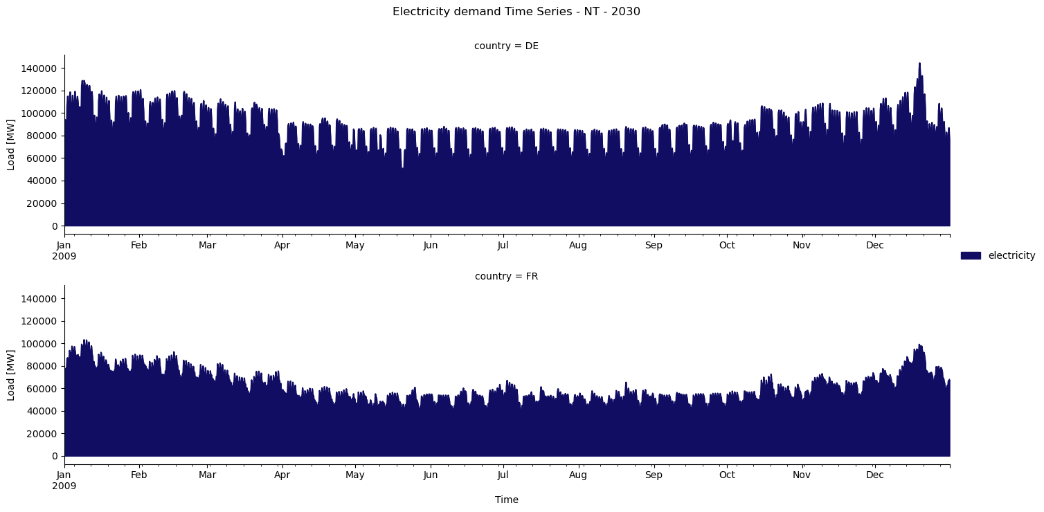
As you can see, the statistics module is a powerful tool to explore your results. You can find more information about it in the first workshop notebook and in the official PyPSA documentation.
PECD capacity factors#
The Pan-European Climate Database (PECD) provides capacity factor profiles for all the different renewable technologies used in the TYNDP. We processed these input data files into a Python and PyPSA friendly input format.
Let’s start by looking at the processed capacity factor time series for Solar PV Rooftop for 2030. These processed data are stored in the resources directory, as they are an output of build_renewable_profiles_pecd. We will filter the data to a set of countries and a week.
cf_pv_rftp = pd.read_csv(
    "resources/tyndp/NT/pecd_data_LFSolarPVRooftop_2030.csv",
    index_col=0,
    parse_dates=True,
).loc["2009-07-01":"2009-07-04", ["SE04", "DE00", "FR00", "ES00"]]
cf_pv_rftp.head(10)
| SE04 | DE00 | FR00 | ES00 | |
|---|---|---|---|---|
| 2009-07-01 00:00:00 | 0.000000 | 0.000000 | 0.000000 | 0.000000 |
| 2009-07-01 01:00:00 | 0.000000 | 0.000000 | 0.000000 | 0.000000 |
| 2009-07-01 02:00:00 | 0.000000 | 0.000000 | 0.000000 | 0.000000 |
| 2009-07-01 03:00:00 | 0.000675 | 0.000000 | 0.000000 | 0.000000 |
| 2009-07-01 04:00:00 | 0.025404 | 0.014742 | 0.000006 | 0.000000 |
| 2009-07-01 05:00:00 | 0.089659 | 0.080133 | 0.012409 | 0.000161 |
| 2009-07-01 06:00:00 | 0.219141 | 0.183108 | 0.103228 | 0.036403 |
| 2009-07-01 07:00:00 | 0.335188 | 0.302943 | 0.273422 | 0.193056 |
| 2009-07-01 08:00:00 | 0.434071 | 0.410089 | 0.435672 | 0.378127 |
| 2009-07-01 09:00:00 | 0.508352 | 0.489067 | 0.559419 | 0.533209 |
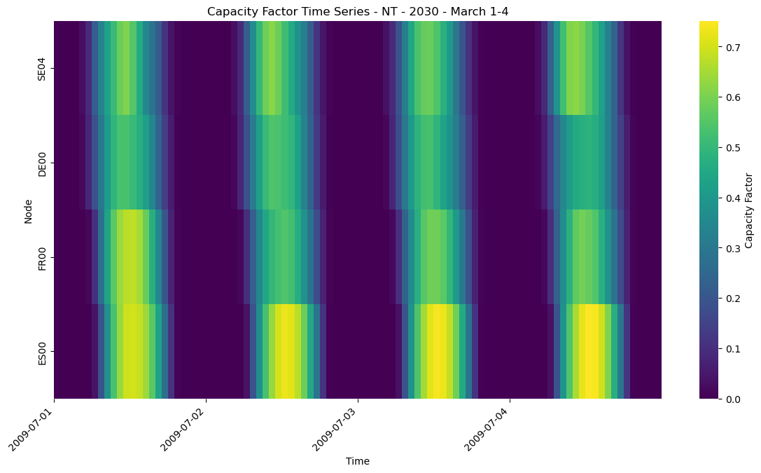
Using a heatmap, we can better grasp the content of the data.
fig, ax = plt.subplots()
sns.heatmap(cf_pv_rftp.T, cmap="viridis", cbar_kws={"label": "Capacity Factor"}, ax=ax)

ax.set_title("Capacity Factor Time Series - NT - 2030 - March 1-4")
tick_positions = range(0, len(cf_pv_rftp), 24)
ax.set_xticks(tick_positions)
ax.set_xticklabels(
    cf_pv_rftp.index[tick_positions].strftime("%Y-%m-%d"), rotation=45, ha="right"
)

ax.set_xlabel("Time")
ax.set_ylabel("Node");
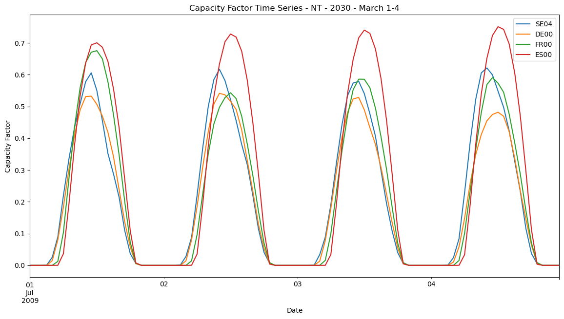
We can also present the data in a line plot.
fig, ax = plt.subplots()

cf_pv_rftp.plot(
    title="Capacity Factor Time Series - NT - 2030 - March 1-4",
    xlabel="Date",
    ylabel="Capacity Factor",
    ax=ax,
);
Task 3: Compute average capacity factor#
a) Locate the resource file with onshore wind capacity factors used for NT in 2030.
b) Compute the average onshore wind capacity factor for all the countries in the PECD.
c) Verify one of the values directly in the network.
Hint: Capacity factors are defined as time-varying parameters of generators and are called p_max_pu.
# Your solution a)
# Your solution b)
# Your solution c)
Onshore wind and solar#
The TYNDP provides existing capacities with the Pan-European Market Modelling database (PEMMDB) and expansion trajectories for given investment candidates and expandable technologies. For the implemented onshore wind and solar technologies, these have been included in beta release v0.3 of the Open-TYNDP model.
It is possible to retrieve those values from the networks as they are added as p_nom_min and p_nom_max of the generators. However, for simplicity, we will import the values directly from the processed input files for the DE scenario. This allows us to investigate the entire trajectory path at once instead of reading one network per planning horizon.
trj = pd.read_csv("resources/tyndp/DE/tyndp_trajectories.csv", index_col=0)
trj.head()
| index_carrier | bus | scenario | pyear | p_nom_min | p_nom_max | |
|---|---|---|---|---|---|---|
| carrier | ||||||
| nuclear | nuclear | AL00 | DE | 2030 | 0.0 | 0.0 |
| nuclear | nuclear | AL00 | DE | 2035 | 0.0 | 0.0 |
| nuclear | nuclear | AL00 | DE | 2040 | 0.0 | 0.0 |
| nuclear | nuclear | AL00 | DE | 2045 | 0.0 | 0.0 |
| nuclear | nuclear | AL00 | DE | 2050 | 0.0 | 0.0 |
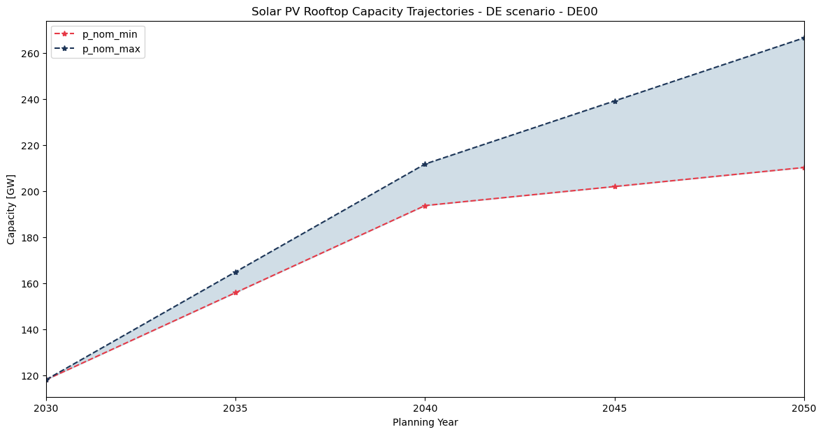
Similar to the capacity factor time series, we want to focus on the Solar PV Rooftop technology and its trajectory path. Let’s take Germany (DE00) to investigate.
trj_pv_rftp_de = (
    trj.query("carrier == 'solar-pv-rooftop' and bus == 'DE00'")
    .sort_values(by="pyear")
    .set_index("pyear")[["p_nom_min", "p_nom_max"]]
    .div(1e3)  # GW
)
trj_pv_rftp_de
| p_nom_min | p_nom_max | |
|---|---|---|
| pyear | ||
| 2030 | 117.998902 | 117.998902 |
| 2035 | 155.874355 | 164.909835 |
| 2040 | 193.749808 | 211.820767 |
| 2045 | 202.028557 | 239.258360 |
| 2050 | 210.307306 | 266.695952 |
Now that we have collected the data, we can create a nice visualization of it.
fig, ax = plt.subplots()
trj_pv_rftp_de.plot(
    title="Solar PV Rooftop Capacity Trajectories - DE scenario - DE00",
    xlabel="Planning Year",
    ylabel="Capacity [GW]",
    color=["#E63946", "#1D3557"],
    style="*--",
    ax=ax,
)

ax.fill_between(
    trj_pv_rftp_de.index,
    trj_pv_rftp_de.iloc[:, 0],
    trj_pv_rftp_de.iloc[:, 1],
    alpha=0.25,
    color="#457B9D",
    label="Trajectory Range",
)

ax.xaxis.set_major_locator(MultipleLocator(5))
ax.set_xlim(trj_pv_rftp_de.index.min(), trj_pv_rftp_de.index.max())
(2030.0, 2050.0)
Now, let’s access the network for the DE scenario to compare one of these trajectory values for 2040.
trj_pv_rftp_de_nc = (
    n_DE_2040.generators.query("carrier == 'solar-pv-rooftop' and bus == 'DE00'")
    .sort_index()[["p_nom_opt", "p_nom_min", "p_nom_max"]]
    .div(1e3)  # in GW
)
trj_pv_rftp_de_nc
| p_nom_opt | p_nom_min | p_nom_max | |
|---|---|---|---|
| name | |||
| DE00 0 solar-pv-rooftop-2030 | 117.998902 | 117.998902 | 117.998902 |
| DE00 0 solar-pv-rooftop-2040 | 75.750906 | 75.750906 | 93.821865 |
Assets remain in the PyPSA network throughout their entire operational lifetime. The year in an asset’s name (e.g “2030”) indicates its build year, not the cumulative capacity in that investment period.
Example: In the 2040 planning year, your network contains:
Generators named “2030” (built in 2030, still operational)
Generators named “2040” (newly built in 2040)
Each generator stores information that depends on its build year (such as efficiency and costs), and after optimization, it contains the cost-optimal capacity that is added in that specific year.
As we can see, the p_nom_min and p_nom_max values for 2040 do not match the reported trajectory values above. The TYNDP trajectories are cumulative trajectories. This means that 2040 generators are bound to extend the optimal capacity of the still operational generators of 2030.
Therefore, if we add the existing capacity (p_nom_opt) from 2030 to the p_nom_min and p_nom_max values from 2040, we will obtain the reported trajectory values shown above:
(
    trj_pv_rftp_de_nc.loc["DE00 0 solar-pv-rooftop-2040", ["p_nom_min", "p_nom_max"]]
    + trj_pv_rftp_de_nc.loc["DE00 0 solar-pv-rooftop-2030", "p_nom_opt"]
)
p_nom_min    193.749808
p_nom_max    211.820767
Name: DE00 0 solar-pv-rooftop-2040, dtype: float64
Task 4: Verify onshore wind trajectories#
Verify onshore wind trajectories in the network itself.
Hint: This can be quick if you can copy and reuse the existing code used above.
# Your solution
Offshore Hubs#
To implement the offshore methodology, new carriers (i.e., technologies) are introduced. All the offshore technologies start with offwind.
offwind_carriers = n_NT_2030.carriers.query("index.str.contains('offwind')")
offwind_carriers_i = offwind_carriers.index
offwind_carriers
| co2_emissions | color | nice_name | max_growth | max_relative_growth | |
|---|---|---|---|---|---|
| name | |||||
| offwind-h2-fl-oh | 0.0 | #9d4d96 | offwind-h2-fl-oh | inf | 0.0 |
| offwind-dc-fb-r | 0.0 | #71b5ed | offwind-dc-fb-r | inf | 0.0 |
| offwind-h2-fb-oh | 0.0 | #c47dbd | offwind-h2-fb-oh | inf | 0.0 |
| offwind-dc-fl-r | 0.0 | #94d4f6 | offwind-dc-fl-r | inf | 0.0 |
| offwind-dc-fb-oh | 0.0 | #74c6f2 | offwind-dc-fb-oh | inf | 0.0 |
| offwind-ac-fl-r | 0.0 | #6da5e8 | offwind-ac-fl-r | inf | 0.0 |
| offwind-dc-fl-oh | 0.0 | #b5e2fa | offwind-dc-fl-oh | inf | 0.0 |
| offwind-ac-fb-r | 0.0 | #6895dd | offwind-ac-fb-r | inf | 0.0 |
As you can see in the table above, all the offshore technologies are implemented. We model technologies that are a combination of the following:
both
acanddczones, as well ash2generating windfarms;both fixed-bottom (
fb) and floating (fl) foundations;both radial (
r) and hub (oh) connections.
We also introduce new offshore buses, both for electricity and hydrogen. Electricity buses use AC_OH as the carrier, while hydrogen buses use H2_OH.
n_NT_2030.buses.query("carrier.str.contains('OH')").head()
| v_nom | type | x | y | carrier | unit | location | v_mag_pu_set | v_mag_pu_min | v_mag_pu_max | control | generator | sub_network | country | substation_lv | substation_off | |
|---|---|---|---|---|---|---|---|---|---|---|---|---|---|---|---|---|
| name | ||||||||||||||||
| BEIOH01 | 380.0 | Hub | 15.199463 | 55.095104 | AC_OH | MWh_el | BEIOH01 | 1.0 | 0.0 | inf | PQ | BE | NaN | NaN | ||
| BEOH001 | 380.0 | Hub | 2.706047 | 51.466411 | AC_OH | MWh_el | BEOH001 | 1.0 | 0.0 | inf | PQ | BE | NaN | NaN | ||
| DEOH001 | 380.0 | FarShoreHub | 6.236433 | 54.812295 | AC_OH | MWh_el | DEOH001 | 1.0 | 0.0 | inf | PQ | DE | NaN | NaN | ||
| DEOH002 | 380.0 | Hub | 13.272319 | 54.471376 | AC_OH | MWh_el | DEOH002 | 1.0 | 0.0 | inf | PQ | DE | NaN | NaN | ||
| DKWOH01 | 380.0 | FarShoreHub | 5.991189 | 56.185492 | AC_OH | MWh_el | DKWOH01 | 1.0 | 0.0 | inf | PQ | DK | NaN | NaN |
Let’s narrow down this list to a single country.
buses = n_NT_2030.buses.query("carrier.str.contains('OH') and country=='BE'")
buses_i = buses.index
buses
| v_nom | type | x | y | carrier | unit | location | v_mag_pu_set | v_mag_pu_min | v_mag_pu_max | control | generator | sub_network | country | substation_lv | substation_off | |
|---|---|---|---|---|---|---|---|---|---|---|---|---|---|---|---|---|
| name | ||||||||||||||||
| BEIOH01 | 380.0 | Hub | 15.199463 | 55.095104 | AC_OH | MWh_el | BEIOH01 | 1.0 | 0.0 | inf | PQ | BE | NaN | NaN | ||
| BEOH001 | 380.0 | Hub | 2.706047 | 51.466411 | AC_OH | MWh_el | BEOH001 | 1.0 | 0.0 | inf | PQ | BE | NaN | NaN | ||
| BEIOH01 H2 | 1.0 | Hub | 15.199463 | 55.095104 | H2_OH | MWh_LHV | BEIOH01 | 1.0 | 0.0 | inf | PQ | BE | NaN | NaN | ||
| BEOH001 H2 | 1.0 | Hub | 2.706047 | 51.466411 | H2_OH | MWh_LHV | BEOH001 | 1.0 | 0.0 | inf | PQ | BE | NaN | NaN |
Using n.plot.explore(), we can easily get an overview of the network topology. Let’s clean the network before exploring it to only focus on the electrical offshore topology.
n_explore_ac_oh = n_NT_2030.copy()
n_explore_ac_oh.remove(
    "Bus", n_explore_ac_oh.buses.query("carrier not in ['AC_OH']").index
)
n_explore_ac_oh.plot.explore()
WARNING:pypsa.plot.maps.interactive:Dropping 1824 row(s) in 'Link' with missing buses
Now, we can search the network for generators that are defined with those carriers.
n_NT_2030.generators.query("carrier in @offwind_carriers_i").head()
| bus | control | type | p_nom | p_nom_mod | p_nom_extendable | p_nom_min | p_nom_max | p_nom_set | p_min_pu | ... | up_time_before | down_time_before | ramp_limit_up | ramp_limit_down | ramp_limit_start_up | ramp_limit_shut_down | weight | p_nom_opt | efficiency_dc_to_b0 | efficiency_dc_to_h2 | |
|---|---|---|---|---|---|---|---|---|---|---|---|---|---|---|---|---|---|---|---|---|---|
| name | |||||||||||||||||||||
| DEOH001 0 offwind-dc-fb-oh-2030 | DEOH001 | PQ | 18868.000000 | 0.0 | False | 18868.000000 | 62868.000000 | NaN | 0.0 | ... | 1 | 0 | NaN | NaN | NaN | NaN | 1.0 | 18868.000000 | 1.0 | 0.68 | |
| NLOR001 0 offwind-dc-fb-r-2030 | NL00 | PQ | 14300.000000 | 0.0 | False | 14300.000000 | 29421.362456 | NaN | 0.0 | ... | 1 | 0 | NaN | NaN | NaN | NaN | 1.0 | 14300.000000 | 1.0 | 0.68 | |
| PLOH001 0 offwind-ac-fb-r-2030 | PL00 | PQ | 9380.015208 | 0.0 | False | 9380.015208 | 9380.015208 | NaN | 0.0 | ... | 1 | 0 | NaN | NaN | NaN | NaN | 1.0 | 9380.015208 | 1.0 | 0.68 | |
| GBOR001 0 offwind-ac-fb-r-2030 | GB00 | PQ | 8975.976664 | 0.0 | False | 8975.976664 | 8975.976664 | NaN | 0.0 | ... | 1 | 0 | NaN | NaN | NaN | NaN | 1.0 | 8975.976664 | 1.0 | 0.68 | |
| GBOR001 0 offwind-dc-fb-r-2030 | GB00 | PQ | 8528.778032 | 0.0 | False | 8528.778032 | 22023.495767 | NaN | 0.0 | ... | 1 | 0 | NaN | NaN | NaN | NaN | 1.0 | 8528.778032 | 1.0 | 0.68 |
5 rows × 44 columns
Let’s focus on a specific country:
n_NT_2030.generators.query("carrier in @offwind_carriers_i and bus in @buses_i")
| bus | control | type | p_nom | p_nom_mod | p_nom_extendable | p_nom_min | p_nom_max | p_nom_set | p_min_pu | ... | up_time_before | down_time_before | ramp_limit_up | ramp_limit_down | ramp_limit_start_up | ramp_limit_shut_down | weight | p_nom_opt | efficiency_dc_to_b0 | efficiency_dc_to_h2 | |
|---|---|---|---|---|---|---|---|---|---|---|---|---|---|---|---|---|---|---|---|---|---|
| name | |||||||||||||||||||||
| BEIOH01 0 offwind-dc-fb-oh-2030 | BEIOH01 | PQ | 3000.000000 | 0.0 | False | 3000.000000 | 12815.264163 | NaN | 0.0 | ... | 1 | 0 | NaN | NaN | NaN | NaN | 1.0 | 3000.000000 | 1.00 | 0.68 | |
| BEOH001 0 offwind-dc-fb-oh-2030 | BEOH001 | PQ | 2647.515945 | 0.0 | False | 2647.515945 | 4847.515945 | NaN | 0.0 | ... | 1 | 0 | NaN | NaN | NaN | NaN | 1.0 | 2647.515945 | 1.00 | 0.68 | |
| BEOH001 0 offwind-h2-fb-oh-2030 | BEOH001 H2 | PQ | 0.000000 | 0.0 | False | 0.000000 | 3296.310843 | NaN | 0.0 | ... | 1 | 0 | NaN | NaN | NaN | NaN | 1.0 | 0.000000 | 0.68 | 0.68 | |
| BEIOH01 0 offwind-h2-fb-oh-2030 | BEIOH01 H2 | PQ | 0.000000 | 0.0 | False | 0.000000 | 8714.379631 | NaN | 0.0 | ... | 1 | 0 | NaN | NaN | NaN | NaN | 1.0 | 0.000000 | 0.68 | 0.68 |
4 rows × 44 columns
Task 5: Extract existing offshore capacities#
Extract existing offshore capacities for the country of your choice using the statistics module.
# Your solution
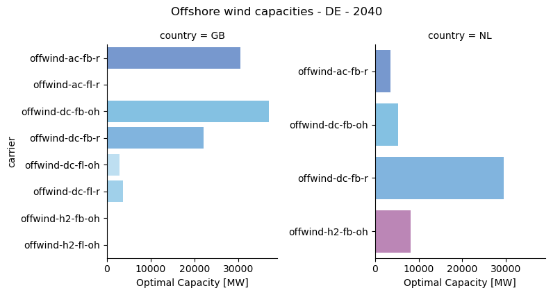
We can also explore the data with the statistics module. First, we can create bar charts.
fig, ax, facet_grid = s_DE_2040.optimal_capacity.plot.bar(
    bus_carrier=["AC", "AC_OH", "H2_OH"],
    query="carrier.str.startswith('offwind') and country in ['NL', 'GB']",
    facet_col="country",
)
fig.suptitle("Offshore wind capacities - DE - 2040", y=1.05);
Then, we can create maps.
# Let's clean a network copy to only keep offshore data
n_map = n_DE_2040.copy()
n_map.remove("Bus", n_map.buses.query("carrier not in ['AC', 'AC_OH', 'H2_OH']").index)
n_map.remove(
    "Generator", n_map.generators.query("not carrier.str.startswith('offwind')").index
)
n_map.remove("Link", n_map.links.index)
n_map.remove("StorageUnit", n_map.storage_units.index)
# Define map projection
def load_projection(plotting_params):
    proj_kwargs = plotting_params.get("projection", dict(name="EqualEarth"))
    proj_func = getattr(ccrs, proj_kwargs.pop("name"))
    return proj_func(**proj_kwargs)


proj = load_projection(dict(name="EqualEarth"))
# Create the map
subplot_kw = {"projection": proj}
fig, ax = plt.subplots(figsize=(9, 9), subplot_kw=subplot_kw)
n_map.statistics.optimal_capacity.plot.map(
    bus_carrier=["AC", "AC_OH", "H2_OH"],
    ax=ax,
    bus_area_fraction=0.006,
    title="Offshore wind capacities - DE - 2040",
    legend_circles_kw=dict(
        frameon=False,
    ),
);
/home/runner/miniconda3/envs/open-tyndp-workshops/lib/python3.13/site-packages/pypsa/plot/statistics/maps.py:253: UserWarning: When combining n.plot() with other plots on a geographical axis, ensure n.plot() is called first or the final axis extent is set initially (ax.set_extent(boundaries, crs=crs)) for consistent legend circle sizes.
  add_legend_circles(
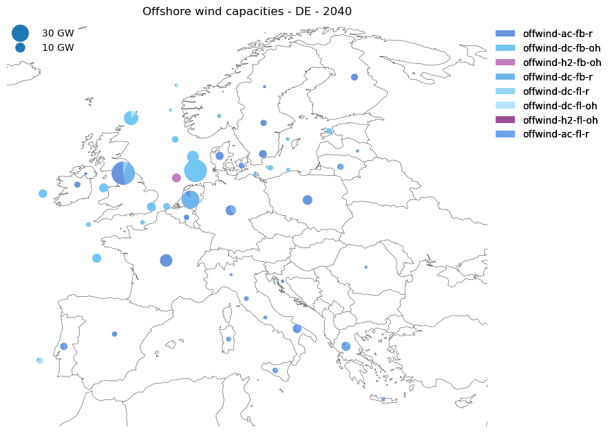
On the map above, we can see the two types of offshore wind connections. Radially connected capacities are attached to and plotted on the mainland node, hence offshore capacities “on land”. In contrast, offshore hub capacities are attached to and plotted on the actual offshore nodes.
The NT scenario is a dispatch scenario. This is implemented in PyPSA using the argument p_nom_extendable = False. However, for the two other scenarios, we need to model capacity expansion.
Currently, the model is configured to do myopic optimization. This means that only the capacities of the current planning horizon are expandable. Generators of the previous planning horizons are fixed at their optimal capacities. Let’s verify this in the network.
# Let's explore offshore wind generators in Denmark
c_buses = n_DE_2040.buses.query("country == 'DK'").index
(
    n_DE_2040.generators.query("carrier in @offwind_carriers_i and bus in @c_buses")[
        [
            "build_year",
            "p_nom",
            "p_nom_min",
            "p_nom_max",
            "p_nom_opt",
            "p_nom_extendable",
        ]
    ].sort_values(by="build_year")
)
| build_year | p_nom | p_nom_min | p_nom_max | p_nom_opt | p_nom_extendable | |
|---|---|---|---|---|---|---|
| name | ||||||
| DKEOR01 0 offwind-ac-fb-r-2030 | 2030 | 1948.858129 | 1948.842756 | 5042.030364 | 1948.858129 | False |
| DKEOR01 0 offwind-dc-fb-r-2030 | 2030 | 579.357244 | 579.357244 | 579.357244 | 579.357244 | False |
| DKWOR01 0 offwind-ac-fb-r-2030 | 2030 | 2722.421378 | 2722.400000 | 24975.197950 | 2722.421378 | False |
| DKWOH01 0 offwind-dc-fb-oh-2040 | 2040 | 14000.000000 | 14000.000000 | 59983.343624 | 14000.004783 | True |
| BEIOH01 0 offwind-ac-fb-r-2040 | 2040 | 0.000000 | 0.000000 | 478.548229 | 0.002418 | True |
| DKWOR01 0 offwind-ac-fb-r-2040 | 2040 | 3999.978622 | 3999.978622 | 22252.776572 | 3999.978624 | True |
| DKEOR01 0 offwind-ac-fb-r-2040 | 2040 | 999.984626 | 999.984626 | 3093.172235 | 999.985204 | True |
| DKEOR01 0 offwind-dc-fb-r-2040 | 2040 | 0.000000 | 0.000000 | 0.000000 | 0.000000 | True |
| DKWOR01 0 offwind-dc-fb-r-2040 | 2040 | 0.000000 | 0.000000 | 23617.979645 | 0.002202 | True |
| DKWOR01 0 offwind-dc-fl-r-2040 | 2040 | 0.000000 | 0.000000 | 1669.878780 | 0.001664 | True |
| DKWOH01 0 offwind-h2-fb-oh-2040 | 2040 | 0.000000 | 0.000000 | 40788.673665 | 0.001980 | True |
You can see multiple columns in the table:
build_year, the build year of the asset (input)p_nom, the nominal power (input)p_nom_min, if expansion is enabled, the minimum value of the nominal capacity (input)p_nom_max, if expansion is enabled, the maximum value of the nominal capacity (input)p_nom_opt, the optimized nominal capacity (output)p_nom_extendable, if expansion is enabled for that asset (input)
The p_nom_min reflects the existing capacities defined in the TYNDP, while the p_nom_max represents the layer potential. We also implemented constraints to ensure we respect the zone potentials and the trajectories defined in the data:
A constraint limits the expansion of DC and H2 sitting on the same location, as the sum of the two capacities cannot exceed the layer potential.
A constraint sets the maximum potential per zone, taking into account the zone trajectories.
H2 imports#
There have also been some important additions to the H2 infrastructure since our last workshop. The different H2 import corridors are now included in the model with a simple pipeline transport representation, similar to the H2 reference grid.
The import pipelines are implemented using PyPSA’s link component. As is convention in PyPSA, this means bus0 represents the external import node and bus1 the importing country’s Hydrogen Zone 2 node.
We can investigate our NT network and list the importing nodes.
h2_import = n_NT_2030.links.filter(like="H2 import", axis=0)
set(h2_import.bus1)
{'BE H2 Z2',
 'DE H2 Z2',
 'ES H2 Z2',
 'FR H2 Z2',
 'HU H2 Z2',
 'IT H2 Z2',
 'NL H2 Z2',
 'RO H2 Z2',
 'SK H2 Z2'}
As we can see from the p_nom_extendable attribute of these links, the H2 import corridors cannot be endogenously expanded by the model but are rather fixed inputs as in the TYNDP 2024 methodology.
h2_import.p_nom_extendable.all()
np.False_
h2_import[["bus0", "bus1", "carrier", "p_nom_extendable"]].head()
| bus0 | bus1 | carrier | p_nom_extendable | |
|---|---|---|---|---|
| name | ||||
| H2 import DZ -> ES - low | DZ-ES-LOW H2 import | ES H2 Z2 | H2 import Pipeline | False |
| H2 import DZ -> ES - high | DZ-ES-HIGH H2 import | ES H2 Z2 | H2 import Pipeline | False |
| H2 import MA -> ES - low | MA-ES-LOW H2 import | ES H2 Z2 | H2 import Pipeline | False |
| H2 import MA -> ES - high | MA-ES-HIGH H2 import | ES H2 Z2 | H2 import Pipeline | False |
| H2 import DZ -> IT - low | DZ-IT-LOW H2 import | IT H2 Z2 | H2 import Pipeline | False |
We can investigate our DE network to create a similar plot to what we created last time. Let’s import some handy plotting functions from the open-tyndp workflow for this:
# It is generally NOT a recommended practice to ignore deprecation warnings.
# However, for the purposes of this workshop, we will make use of it to make our output less noisy
warnings.filterwarnings(action="ignore", category=DeprecationWarning)
from scripts.plot_base_hydrogen_network import plot_h2_map_base
And plot the H2 reference grid together with the import corridors:
warnings.filterwarnings(action="ignore", category=DeprecationWarning)
map_opts = {
    "boundaries": [-11, 30, 28, 71],
    "geomap_colors": {
        "ocean": "white",
        "land": "white",
    },
}

plot_h2_map_base(
    network=n_DE_2040,
    map_opts=map_opts,
    map_fn="../../../h2_import_corridors_DE2040.png",
)
Image("../../../h2_import_corridors_DE2040.png")
INFO:scripts.plot_base_hydrogen_network:Plotting base H2 pipeline and import capacities.
/home/runner/work/open-tyndp-workshops/open-tyndp-workshops/open-tyndp-workshops/data/open-tyndp-20251016/scripts/plot_base_hydrogen_network.py:205: UserWarning: When combining n.plot() with other plots on a geographical axis, ensure n.plot() is called first or the final axis extent is set initially (ax.set_extent(boundaries, crs=crs)) for consistent legend circle sizes.
  add_legend_circles(
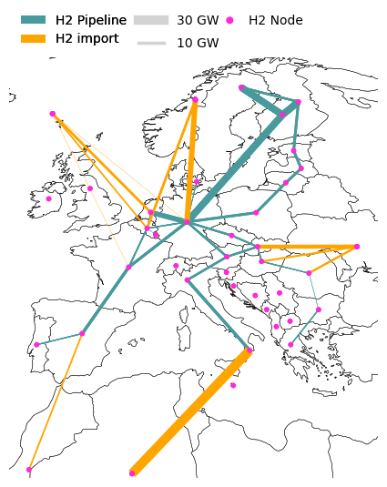
Task 6: Investigate H2 import corridors#
a) Extract and investigate the different import corridors for one specific country of your choice using our NT 2030 network.
b) Compare with DE 2040 data.
# Your solution a)
# Your solution b)
Benchmarking framework#
Open-TYNDP introduces a benchmarking framework for continuous and systematic validation of Open-TYNDP model outputs against TYNDP 2024 scenarios. This framework provides flexible and scalable validation across multiple metrics and benchmarking methods.
Comprehensive documentation of the framework can be found in the documentation.
Metrics#
The following metrics from the TYNDP 2024 Scenarios report are considered relevant for benchmarking:
Exogenous Inputs:
Benchmark Final Energy demand by fuel, EU27 (TWh), (Fig 5, p24 and Fig 51, p63)
Benchmark Electricity demand per sector, EU27 (TWh), (Fig 6, p25 and Fig 52, p63)
Benchmark Methane demand by sector, EU27 (TWh), (Fig 8, p27 and Fig 53, p64)
Benchmark Hydrogen demand by sector, EU27 (TWh), (Fig 10, p28 and Fig 54, p64)
Investment and dispatch modelling outputs:
Benchmark of net installed capacity for electricity generation, EU27 (GW), (Fig 25, p39 and Fig 55, p65)
Benchmark of electricity generation, EU27 (TWh), (Fig 26, p39 and Fig 56, p65)
Benchmark methane supply, EU27 (TWh), (Fig 32, p45 and Fig 57, p66)
Benchmark hydrogen supply, EU27 (TWh), (Fig 33, p46 and Fig 58, p67)
Benchmark biomass supply, EU27 (TWh), (Fig 59, p67)
Benchmark energy imports, EU27 (TWh), (Fig 40, p51 and Fig 60, p68)
Hourly generation profile of power generation, Fig 30, p35
The benchmarking is based on a methodology proposed by Wen et al. (2022). This methodology provides a multi-criteria approach to ensure: diversity, effectiveness, robustness, and compatibility.
This methodology defines the following indicators:
Missing: Count of carriers/sectors dropped due to missing values
sMPE (Symmetric Mean Percentage Error): Indicates the direction of the deviation between modeled scenarios and TYNDP 2024 outcomes, showing if the output is overall overestimated or underestimated.
sMAPE (Symmetric Mean Absolute Percentage Error): Indicates the absolute magnitude of the deviations, avoiding the cancellation of negative and positive errors.
sMdAPE (Symmetric Median Absolute Percentage Error): Provides skewness information to complement sMAPE.
RMSLE (Root Mean Square Logarithmic Error): Complements the percentage errors since it shows the logarithmic deviation values.
Growth error: Shows the error on the temporal scale (i.e., between planning horizons). This indicator is ignored for dynamic time series (i.e., hourly generation profiles).
Outputs#
Warning
Open-TYNDP is under active development and is not yet feature-complete. The current development status and the general Limitations are important to understand before assessing the current benchmarking results.
We can now explore the content of the results/tyndp/<SCENARIO>/validation folder. It’s in this folder that all the benchmarking data is stored. First, let’s have a look at the summary figure. This figure presents the magnitude of the error for all indicators.
display(
    convert_from_path("results/tyndp/NT/validation/kpis_eu27_s_all___all_years.pdf")[0]
)
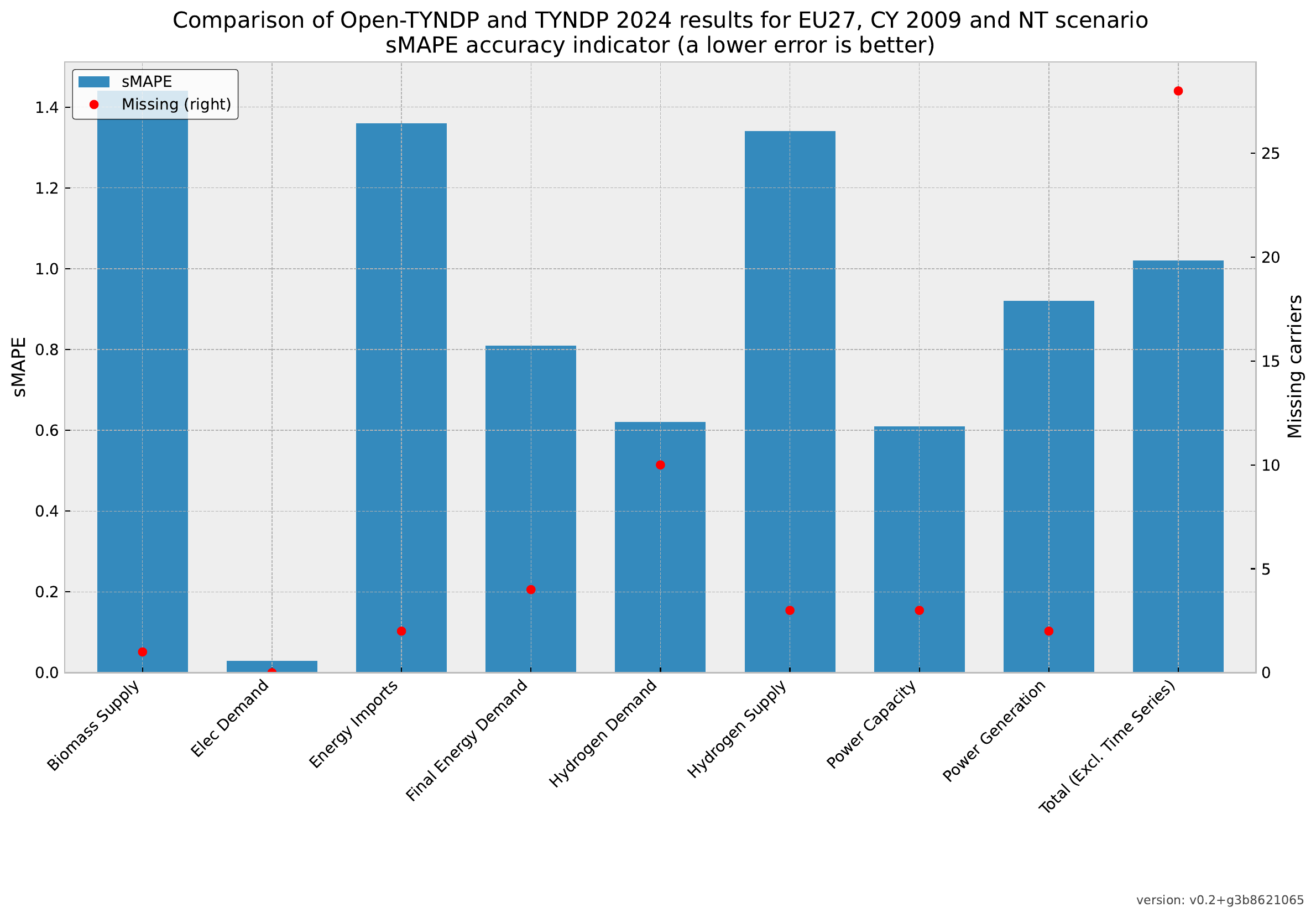
Associated with this figure, a table presents all the indicators for each metric.
pd.read_csv("results/tyndp/NT/validation/kpis_eu27_s_all___all_years.csv", index_col=0)
| sMPE | sMAPE | sMdAPE | RMSLE | Growth Error | Missing | version | |
|---|---|---|---|---|---|---|---|
| biomass_supply | -1.44 | 1.44 | 1.44 | 4.42 | 0.52 | 1.0 | v0.2+g3b8621065 |
| elec_demand | 0.03 | 0.03 | 0.03 | 0.03 | 0.00 | 0.0 | v0.2+g3b8621065 |
| energy_imports | -1.30 | 1.36 | 2.00 | 27.07 | 0.16 | 2.0 | v0.2+g3b8621065 |
| final_energy_demand | -0.77 | 0.81 | 0.96 | 1.27 | 0.02 | 4.0 | v0.2+g3b8621065 |
| generation_profiles | NaN | NaN | NaN | NaN | NaN | NaN | v0.2+g3b8621065 |
| hydrogen_demand | -0.27 | 0.62 | 0.53 | 0.74 | NaN | 10.0 | v0.2+g3b8621065 |
| hydrogen_supply | -1.00 | 1.34 | 1.63 | 11.35 | 0.04 | 3.0 | v0.2+g3b8621065 |
| methane_demand | NaN | NaN | NaN | NaN | NaN | NaN | v0.2+g3b8621065 |
| methane_supply | NaN | NaN | NaN | NaN | NaN | NaN | v0.2+g3b8621065 |
| power_capacity | -0.39 | 0.61 | 0.40 | 2.61 | -0.00 | 3.0 | v0.2+g3b8621065 |
| power_generation | -0.25 | 0.92 | 0.67 | 3.01 | -0.01 | 2.0 | v0.2+g3b8621065 |
| Total (excl. time series) | -0.65 | 1.02 | 0.90 | 8.25 | 0.02 | 28.0 | v0.2+g3b8621065 |
Note that figures and tables will always include a version tag (in this case v0.2+gb9516f6f1) to clearly identify the version of the codebase used to produce the validation.
The same benchmarking information is available for all the metrics. Let’s explore the quality of the power capacity metric.
display(
    convert_from_path(
        "results/tyndp/NT/validation/graphics_s_all___all_years/benchmark_power_capacity_eu27_cy2009_2030.pdf"
    )[0]
)
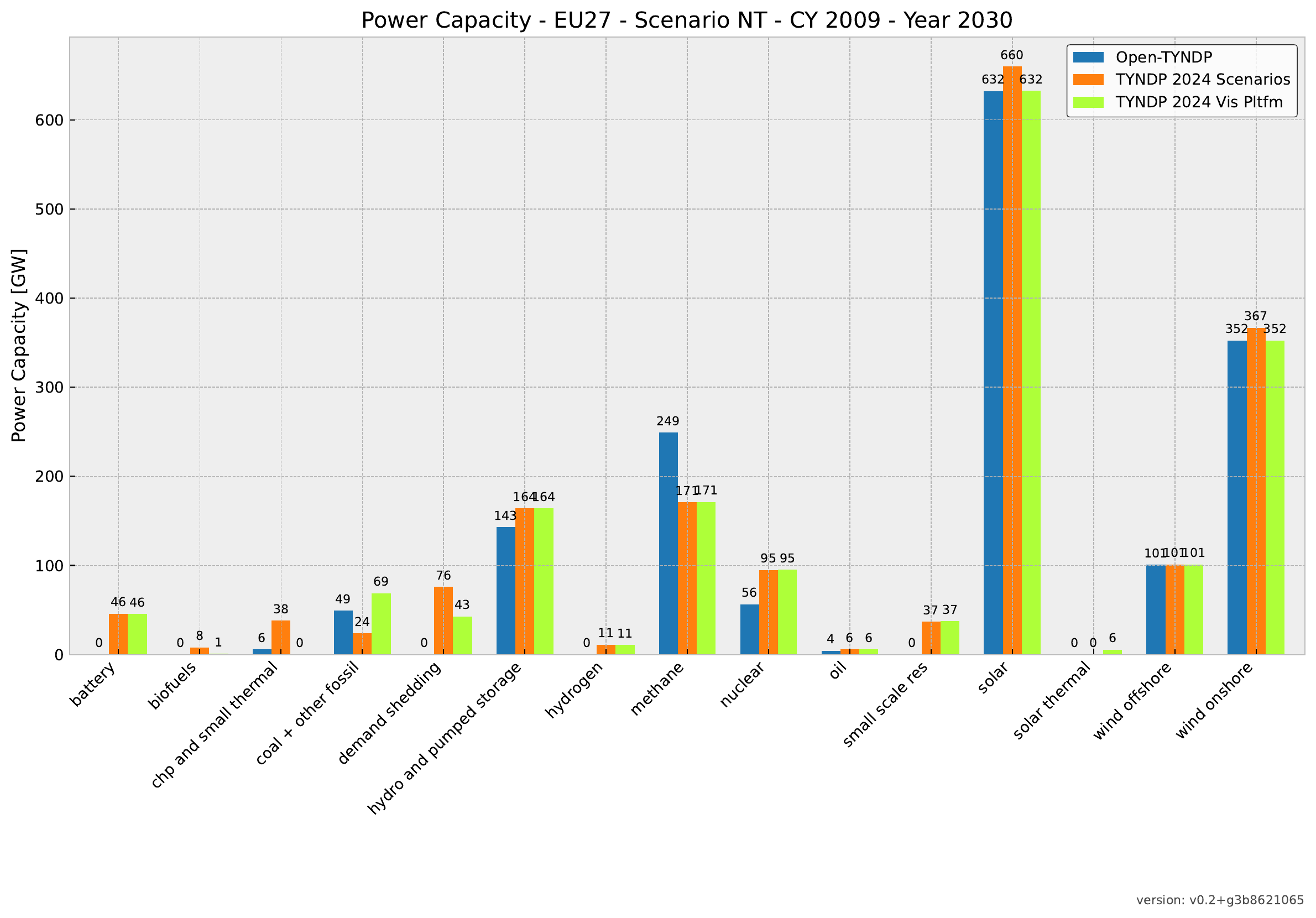
Again, a table associated with the figure shows the detailed benchmarking data.
pd.read_csv(
    "results/tyndp/NT/validation/csvs_s_all___all_years/power_capacity_eu27_cy2009_s_all___all_years.csv",
    index_col=0,
)
| sMPE | sMAPE | sMdAPE | RMSLE | Growth Error | version | |
|---|---|---|---|---|---|---|
| battery | -1.33 | 1.33 | 1.33 | 3.35 | 0.39 | v0.2+g3b8621065 |
| chp and small thermal | -1.67 | 1.67 | 1.67 | 2.83 | -0.17 | v0.2+g3b8621065 |
| coal + other fossil | 0.56 | 0.56 | 0.56 | 0.59 | -0.03 | v0.2+g3b8621065 |
| hydro and pumped storage | -0.16 | 0.16 | 0.16 | 0.17 | -0.01 | v0.2+g3b8621065 |
| hydrogen | -1.24 | 1.24 | 1.24 | 7.35 | 0.99 | v0.2+g3b8621065 |
| methane | 0.51 | 0.51 | 0.51 | 0.54 | 0.03 | v0.2+g3b8621065 |
| nuclear | -0.81 | 0.81 | 0.81 | 0.97 | -0.07 | v0.2+g3b8621065 |
| oil | -0.08 | 0.27 | 0.27 | 0.29 | 0.05 | v0.2+g3b8621065 |
| solar | -0.05 | 0.05 | 0.05 | 0.05 | -0.00 | v0.2+g3b8621065 |
| wind offshore | -0.00 | 0.00 | 0.00 | 0.00 | 0.00 | v0.2+g3b8621065 |
| wind onshore | -0.05 | 0.05 | 0.05 | 0.06 | -0.00 | v0.2+g3b8621065 |
| biofuels | NaN | NaN | NaN | NaN | NaN | v0.2+g3b8621065 |
| small scale res | NaN | NaN | NaN | NaN | NaN | v0.2+g3b8621065 |
| demand shedding | NaN | NaN | NaN | NaN | NaN | v0.2+g3b8621065 |
This feature is still work in progress and will be improved throughout the project.
Solutions#
Task 1: Executing a workflow with Snakemake#
# Solution a)
# ! snakemake -call data/base_2030.nc -n
# Solution b)
# ! snakemake -call
# Solution c)
# ! snakemake -call
# Solution d)
# Path("data/data_raw.csv").touch()
# ! snakemake -call
# Solution e)
# rule retrieve_data_2:
#     input:
#         "data/data_raw.csv"
#     output:
#         "data/data_raw_2.csv"
#     shell:
#         "cp {input} {output}"
#
# rule build_data_2:
#     input:
#         "data/data_raw_2.csv"
#     output:
#         "data/data_filtered_2.csv"
#     script:
#         "scripts/build_data.py"
#
# rule prepare_network:
#     input:
#         "data/data_filtered.csv",
#         "data/data_filtered_2.csv"
#     output:
#         "data/base_2030.nc"
#     script:
#         "scripts/prepare_network.py"
Task 2: Explore the folder#
# Solution a)
# data/tyndp_2024_bundle
# Solution b)
# config/config.tyndp.yaml
# Solution c)
# results/tyndp/NT/maps/base_s_all__-h2_network_2040.pdf
Task 3: Compute average capacity factor#
# Solution a)
cf_onwind = pd.read_csv(
    "resources/tyndp/NT/pecd_data_Wind_Onshore_2030.csv",
    index_col=0,
    parse_dates=True,
)
cf_onwind.head()
| AL00 | AT00 | BA00 | BE00 | BG00 | CH00 | CY00 | CZ00 | DE00 | DKE1 | ... | RO00 | RS00 | SE01 | SE02 | SE03 | SE04 | SI00 | SK00 | ITCO | ITVI | |
|---|---|---|---|---|---|---|---|---|---|---|---|---|---|---|---|---|---|---|---|---|---|
| 2009-01-01 00:00:00 | 0.065672 | 0.085327 | 0.221089 | 0.012502 | 0.180310 | 0.083889 | 0.534456 | 0.163332 | 0.066001 | 0.118449 | ... | 0.120159 | 0.034304 | 0.702190 | 0.642226 | 0.366219 | 0.111668 | 0.128477 | 0.198581 | 0.0 | 0.0 |
| 2009-01-01 01:00:00 | 0.070347 | 0.059715 | 0.250842 | 0.014052 | 0.167783 | 0.096225 | 0.497899 | 0.153907 | 0.079850 | 0.147396 | ... | 0.126642 | 0.032849 | 0.704075 | 0.660711 | 0.392257 | 0.119482 | 0.116763 | 0.170496 | 0.0 | 0.0 |
| 2009-01-01 02:00:00 | 0.077664 | 0.039210 | 0.272526 | 0.015396 | 0.159716 | 0.063696 | 0.435759 | 0.147612 | 0.092935 | 0.157954 | ... | 0.135300 | 0.036249 | 0.719817 | 0.679683 | 0.405772 | 0.123030 | 0.103016 | 0.142045 | 0.0 | 0.0 |
| 2009-01-01 03:00:00 | 0.089141 | 0.030230 | 0.289429 | 0.012973 | 0.157374 | 0.051421 | 0.389443 | 0.141560 | 0.102895 | 0.144227 | ... | 0.146763 | 0.040961 | 0.736409 | 0.701676 | 0.417852 | 0.151473 | 0.086030 | 0.123585 | 0.0 | 0.0 |
| 2009-01-01 04:00:00 | 0.098864 | 0.029790 | 0.297122 | 0.011561 | 0.157447 | 0.058431 | 0.343547 | 0.134129 | 0.117694 | 0.121793 | ... | 0.172136 | 0.054967 | 0.745064 | 0.723927 | 0.423064 | 0.184682 | 0.066500 | 0.104355 | 0.0 | 0.0 |
5 rows × 54 columns
# Solution b)
cf_onwind.columns = cf_onwind.columns.str[:2]
cf_onwind.columns.name = "country"

cf_onwind_sorted = cf_onwind.T.groupby(by="country").mean().mean(axis=1).sort_values()
cf_onwind_sorted.tail()
country
GR    0.345672
GB    0.347628
FI    0.357377
LT    0.369007
IE    0.384240
dtype: float64
fig, ax = plt.subplots(figsize=(14, 9))
cf_onwind_sorted.plot.barh(
    title="Average capacity factors - 2030",
    xlabel="Capacity factor [p.u]",
    ylabel="Country",
    ax=ax,
);
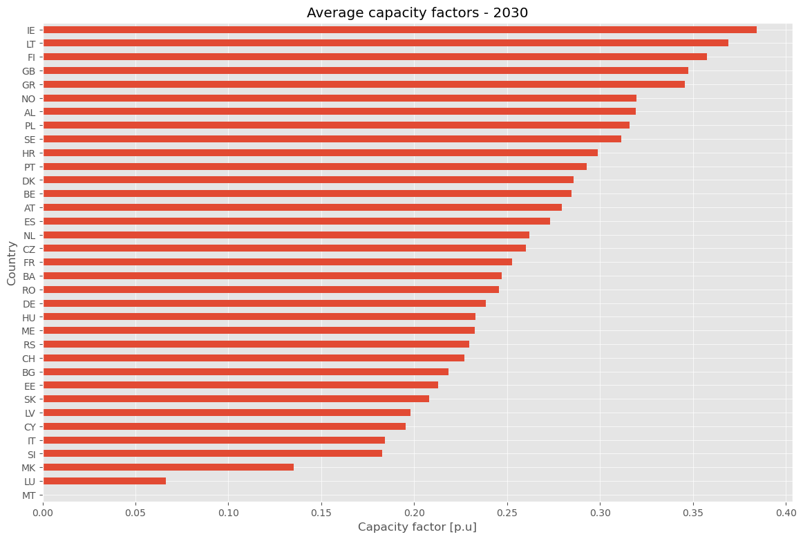
# Solution c)
c_buses = n_NT_2030h.buses.query("country=='IE'").index
c_gen = n_NT_2030h.generators.query("carrier=='onwind' and bus in @c_buses").index
c_cf = n_NT_2030h.generators_t.p_max_pu[c_gen]
c_cf.mean()
name
IE00 0 onwind    0.38424
dtype: float64
Task 4: Verify onshore wind trajectories#
# Solution
(
    pd.read_csv("resources/tyndp/DE/tyndp_trajectories.csv", index_col=0)
    .query("bus=='DE00' and carrier == 'onwind'")
    .set_index("pyear")
    .sort_index()[["p_nom_min", "p_nom_max"]]
    .div(1e3)  # in GW
)
| p_nom_min | p_nom_max | |
|---|---|---|
| pyear | ||
| 2030 | 115.0000 | 115.00 |
| 2035 | 136.9375 | 141.75 |
| 2040 | 158.8750 | 168.50 |
| 2045 | 160.0000 | 180.00 |
| 2050 | 161.1250 | 191.50 |
trj_onwind_de = (
    n_DE_2040.generators.query("carrier == 'onwind' and bus == 'DE00'")
    .sort_index()[["p_nom_opt", "p_nom_min", "p_nom_max"]]
    .div(1e3)  # in GW
)
trj_onwind_de
| p_nom_opt | p_nom_min | p_nom_max | |
|---|---|---|---|
| name | |||
| DE00 0 onwind-2030 | 115.000000 | 115.000 | 115.0 |
| DE00 0 onwind-2040 | 43.875004 | 43.875 | 53.5 |
(
    trj_onwind_de.loc["DE00 0 onwind-2040", ["p_nom_min", "p_nom_max"]]
    + trj_onwind_de.loc["DE00 0 onwind-2030", "p_nom_opt"]
)
p_nom_min    158.875
p_nom_max    168.500
Name: DE00 0 onwind-2040, dtype: float64
Task 5: Extract existing offshore capacities#
# Solution
(
    s_NT_2030.optimal_capacity(
        bus_carrier=["AC", "AC_OH", "H2_OH"],
        comps="Generator",
        groupby=["bus", "carrier"],
    )
    .to_frame("p_nom_opt")
    .query("bus.str.contains('BE') and carrier.str.startswith('offwind')")
)
| p_nom_opt | ||
|---|---|---|
| bus | carrier | |
| BE00 | offwind-ac-fb-r | 3112.484 |
| BEIOH01 | offwind-dc-fb-oh | 3000.000 |
| BEOH001 | offwind-dc-fb-oh | 2647.516 |
Task 6: Investigate H2 import corridors#
# Solution a)
(
    n_NT_2030.links.filter(like="H2 import", axis=0).query("bus1.str.contains('BE')")[
        ["bus0", "bus1", "carrier", "p_nom"]
    ]
)
| bus0 | bus1 | carrier | p_nom | |
|---|---|---|---|---|
| name | ||||
| H2 import NO -> BE - low | NO-BE-LOW H2 import | BE H2 Z2 | H2 import Pipeline | 0.000000 |
| H2 import NO -> BE - high | NO-BE-HIGH H2 import | BE H2 Z2 | H2 import Pipeline | 0.000000 |
| H2 import Ammonia -> BE - low | Ammonia-BE-LOW H2 import | BE H2 Z2 | H2 import LH2 | 2283.105023 |
| H2 import Ammonia -> BE - high | Ammonia-BE-HIGH H2 import | BE H2 Z2 | H2 import LH2 | 0.000000 |
# Solution b)
(
    n_DE_2040.links.filter(like="H2 import", axis=0).query("bus1.str.contains('BE')")[
        ["bus0", "bus1", "carrier", "p_nom"]
    ]
)
| bus0 | bus1 | carrier | p_nom | |
|---|---|---|---|---|
| name | ||||
| H2 import NO -> BE - low | NO-BE-LOW H2 import | BE H2 Z2 | H2 import Pipeline | 2500.000000 |
| H2 import NO -> BE - high | NO-BE-HIGH H2 import | BE H2 Z2 | H2 import Pipeline | 5833.333333 |
| H2 import Ammonia -> BE - low | Ammonia-BE-LOW H2 import | BE H2 Z2 | H2 import LH2 | 5117.580000 |
| H2 import Ammonia -> BE - high | Ammonia-BE-HIGH H2 import | BE H2 Z2 | H2 import LH2 | 0.000000 |
Notebook clean up#
# navigate back into the main working directory
os.chdir("../..")

# Only clean up data when running in CI environment
if os.getenv("CI"):
    rm_dir = "data/open-tyndp-20251016"
    print(
        f"CI environment detected. Cleaning up notebook data by removing '{rm_dir}' and '{rm_dir}.zip'."
    )
    shutil.rmtree(rm_dir, ignore_errors=True)
    Path(f"{rm_dir}.zip").unlink(missing_ok=True)
else:
    print("Skipping cleanup (not in CI environment).")
CI environment detected. Cleaning up notebook data by removing 'data/open-tyndp-20251016' and 'data/open-tyndp-20251016.zip'.