Workshop 4: Open-TYNDP Outcomes and CBA Workflows

Workshop 4: Open-TYNDP Outcomes and CBA Workflows#

Note

At the end of this notebook, you will be able to:

1. Inspect Open-TYNDP benchmarks

Investigate the latest networks using PyPSA-Explorer
Benchmark Open-TYNDP NT scenario outcomes by comparing PyPSA statistical data
Modify assumptions to test alternative scenarios (advanced users)

2. Run CBA workflows

Modify the CBA configuration for the targeted project and/or climate year
Learn how to execute CBA analysis coupled to or detached from the Scenario Building workflow

Warning

This notebook uses pre-downloaded results and runs simplified workflows designed for learning purposes. It is not a substitute for running the full Open-TYNDP workflow. All examples and results are based on Open-TYNDP v0.7.1 — outputs may differ in other versions.

Note

If you have not set up Python on your computer, you can execute this tutorial in your browser via Google Colab. Click the rocket button in the top right corner and launch “Colab”. If that doesn’t work, download the .ipynb file and import it in Google Colab.

Then install the required packages by uncommenting the cell below.

# uncomment for running this notebook on Colab
# !pip install packaging==25.0 --q
# !pip install pypsa==1.2.1 pypsa-explorer pandas matplotlib numpy pdf2image cartopy snakemake
# !apt-get install poppler-utils -qq

# Standard library imports
import os
import shutil
import zipfile
from datetime import datetime
from pathlib import Path
from urllib.request import urlretrieve

import matplotlib.pyplot as plt
import pandas as pd
import pypsa
from pypsa_explorer import create_app

# Plot settings
pypsa.set_option("params.statistics.nice_names", True)
pypsa.set_option("params.statistics.drop_zero", True)
pypsa.set_option("params.statistics.round", 3)
plt.rcParams["figure.figsize"] = [14, 7]
clip = 1  # TWh

We use a custom unzip function here to preserve the original file timestamps. This matters for snakemake, which uses timestamps to decide which files need to be re-run.

def unzip_with_timestamps(zip_path, extract_to, keep_zip=True):
    """Unzip a file while preserving original file timestamps."""
    with zipfile.ZipFile(zip_path, "r") as zip_ref:
        for member in zip_ref.infolist():
            # Extract the file
            zip_ref.extract(member, extract_to)

            # Get the extracted file path
            extracted_path = os.path.join(extract_to, member.filename)

            # Get the modification time from the zip file
            date_time = datetime(*member.date_time)
            timestamp = date_time.timestamp()

            # Set both access and modification times
            os.utime(extracted_path, (timestamp, timestamp))
    if not keep_zip:
        os.remove(zip_path)

We’ll download the latest Open-TYNDP results (v0.7.1) and some helper scripts. The results are pre-computed so you don’t need to run the full optimisation yourself.

urls = {
    "data/results-0.7.1.zip": "https://storage.googleapis.com/open-tyndp-data-store/outcomes/0.7.1/results-0.7.1.zip",
    "scripts/_helpers.py": "https://raw.githubusercontent.com/open-energy-transition/open-tyndp-workshops/refs/heads/main/open-tyndp-workshops/scripts/_helpers.py",
}

if os.path.basename(os.getcwd()) in ["open-tyndp-workshops", "content"]:
    os.makedirs("data", exist_ok=True)
    os.makedirs("scripts", exist_ok=True)
    for name, url in urls.items():
        if os.path.exists(name):
            print(f"File {name} already exists. Skipping download.")
        else:
            print(f"Retrieving {name} from storage.")
            urlretrieve(url, name)
            print(f"File available in {name}.")

    to_dir = "data/results-0.7.1"
    if not os.path.exists(to_dir):
        print(f"Unzipping data/results-0.7.1.zip.")
        unzip_with_timestamps("data/results-0.7.1.zip", "data/results-0.7.1")
    print(f"Latest NT results for Open-TYNDP v0.7.1 are available in '{to_dir}'.")

    print("Done")
else:
    print("Not in open-tyndp-workshops directory.")

Retrieving data/results-0.7.1.zip from storage.

File available in data/results-0.7.1.zip.
File scripts/_helpers.py already exists. Skipping download.
Unzipping data/results-0.7.1.zip.

Latest NT results for Open-TYNDP v0.7.1 are available in 'data/results-0.7.1'.
Done

And we’ll also import some handy helper functions that we introduced in the last workshops.

from scripts._helpers import (
    display_code_lines,
    run_pypsa_explorer_in_colab,
    show_benchmarks,
)

This notebook is running locally !

Scenario Building#

Reminder: Extracting insights from the network#

Let’s load the latest Open-TYNDP NT scenario outcomes (v0.7.1) again and explore them using the PyPSA-Explorer and the PyPSA.statistics module.

# Define the path and an importer function
base_path = "data/results-0.7.1/NT-cy2009-20260520/networks/"


def import_network(fn: str):
    n = pypsa.Network(fn)
    n.sanitize()
    return n


# Load the latest NT scenario networks directly into dictionary for PyPSA-Explorer
networks = {
    "NT 2030": import_network(base_path + "base_s_all___2030.nc"),
    "NT 2040": import_network(base_path + "base_s_all___2040.nc"),
}

WARNING:pypsa.network.io:Importing network from PyPSA version v1.2.1 while current version is v1.2.2. Read the release notes at `https://go.pypsa.org/release-notes` to prepare your network for import.

INFO:pypsa.network.io:Imported network 'PyPSA-Eur (tyndp)' has buses, carriers, generators, global_constraints, links, loads, shapes, storage_units, stores, sub_networks

INFO:pypsa.consistency:Sanitizing network...

INFO:pypsa.components._types.carriers:Assigned colors to 1 carriers using 'tab10' palette.

INFO:pypsa.consistency:Network sanitization complete.

WARNING:pypsa.network.io:Importing network from PyPSA version v1.2.1 while current version is v1.2.2. Read the release notes at `https://go.pypsa.org/release-notes` to prepare your network for import.

INFO:pypsa.network.io:Imported network 'PyPSA-Eur (tyndp)' has buses, carriers, generators, global_constraints, links, loads, shapes, storage_units, stores, sub_networks

INFO:pypsa.consistency:Sanitizing network...

INFO:pypsa.components._types.carriers:Assigned colors to 1 carriers using 'tab10' palette.

INFO:pypsa.consistency:Network sanitization complete.

Interactive Exploration with PyPSA-Explorer#

~20 minutes

As we introduced in the last workshop, PyPSA-Explorer is an interactive dashboard for visualizing and analyzing energy system networks. It provides:

Energy balance analysis with both time series and aggregated views
Capacity planning visualizations by technology and region
Economic analysis showing CAPEX/OPEX breakdowns
Interactive geographical network maps
Support for visualising multiple networks

Reminder: Using the Dashboard#

Once the dashboard opens, you can explore these key features:

1. Energy Balance Tab

View production, consumption, and storage patterns over time
Switch between time series and aggregated views
Filter by energy carrier (electricity, hydrogen, etc.)
Filter by country or region

2. Capacity Tab

Analyze installed capacities across scenarios
Compare capacity buildout between 2030 and 2040
View breakdowns by technology type and region

3. Economics Tab

Examine costs and revenues
Review CAPEX and OPEX breakdowns by technology
Compare regional cost distributions
Assess investment requirements

4. Network Map

Visualize the geographical network layout
View an interactive map with network components
Zoom and pan to explore specific regions

Tip: Use the scenario selector buttons in the top-right corner to switch between NT 2030 and NT 2040 scenarios.

Note

PyPSA-Explorer can be launched in different ways depending on your environment:

Local Jupyter: Use the terminal command (recommended) or inline display
Google Colab: The dashboard launches inline, embedded directly in the notebook

Follow the instructions below for your specific environment.

# Detect if running on Google Colab
try:
    from google.colab import output

    IN_COLAB = True
    print(f"This notebook is running on Google Colab!")
except ImportError:
    IN_COLAB = False
    print(f"This notebook is running locally !")

port = 8050

This notebook is running locally !

For Local Users#

If you’re running locally, we recommend launching PyPSA-Explorer from the terminal for optimal performance:

pypsa-explorer data/results-0.7.1/NT-cy2009-20260520/networks/base_s_all___2030.nc:NT_2030 data/results-0.7.1/NT-cy2009-20260520/networks/base_s_all___2040.nc:NT_2040

This command opens the dashboard in your default browser at http://localhost:8050.

Alternative: The cell below can launch the dashboard inline within the notebook, though the terminal method provides better performance and responsiveness.

# Terminal method recommended
USE_TERMINAL = True  # Change to False if you want to launch from the notebook instead

if not IN_COLAB and not USE_TERMINAL:
    # Local Jupyter: Inline display
    app = create_app(networks)
    app.run(jupyter_mode="tab", port=port, debug=False)

For Google Colab Users#

Running PyPSA-Explorer on Google Colab requires a small workaround to display the dashboard properly inside the notebook.

We already imported a useful helper function we introduced in the last workshop to handle this: run_pypsa_explorer_in_colab()

if IN_COLAB:
    run_pypsa_explorer_in_colab(networks, port)

Tip for Colab users: To view the dashboard in fullscreen mode, click the three dots (⋮) in the top-right corner of the output cell and select “View output fullscreen”.

Task 1: Navigate `PyPSA-Explorer`#

Let’s look at the latest Open-TYNDP NT scenario results (v0.7.1) and explore them interactively using the PyPSA-Explorer. Let’s try to find some specific information about the solved networks.

(a) Can you verify the total amount of wind generated on Danish Offshore Hubs in 2040 at 43.55 TWh?

(b) Can you verify that Germany is the largest net annual importer of H2 in 2040?

Hint: Look for H2 pipeline, H2 Import Pipeline and H2 Import LH2 in the energy balance.

(c) Can you verify the observed correlation between electricity mix and H2 production in Germany for the first week of June in 2040?

Explore NT outcomes using the `PyPSA.statistics` module#

~30 minutes

When Open-TYNDP runs an optimisation, all input data, installed capacities, demand profiles, network topology, technology assumptions, is loaded into a PyPSA network object n. After the optimisation completes, the results are stored in the same network object. This means n contains everything: what went in and what came out.

Since a PyPSA network holds a large amount of detailed information across many components, exploring it directly can be overwhelming. This is where n.statistics comes in: a built-in module that gives you fast, easy access to the most important system-level metrics without having to dig into the raw network data yourself.

n.statistics provides a consistent, high-level API that handles component iteration, port mapping, and carrier grouping automatically.

Tip

n.stats is available as a shorthand alias for n.statistics.

Each method can be called individually or explored via the summary table:

Category	Methods
Costs	`capex()`, `installed_capex()`, `expanded_capex()`, `opex()`, `system_cost()`
Capacity	`installed_capacity()`, `optimal_capacity()`, `expanded_capacity()`, `capacity_factor()`
Energy	`supply()`, `withdrawal()`, `energy_balance()`, `transmission()`, `curtailment()`
Market	`prices()`, `revenue()`, `market_value()`

Every method accepts the same filtering and grouping parameters:

Parameter	Description
`groupby`	String, list, or callable — how to group results (default: `\"carrier\"`)
`groupby_method`	Aggregation function (`\"sum\"` (default), `\"mean\"`, …)
`groupby_time`	`\"sum\"`, `\"mean\"`, or `False` for time series — default varies by method
`components`	Filter to specific component types
`carrier`	Filter by carrier name (internal name)
`bus_carrier`	Filter by the carrier of the bus
`nice_names`	Use human-readable carrier names (default: `True`)

Warning

prices() has a simplified interface — groupby and groupby_time are booleans, and it does not accept carrier or components.

The full PyPSA.statistics API documentation is available in the pypsa documentation. Additionally, you can find two video tutorials on PyPSA meets Earth’s youtube channel (part 1, part 2) for more comprehensive information and examples on how to use the statistics module. This learning material is open-source and available on GitHub.

Reminder: Extracting insights from a network#

To start of we’ll have a look at the network for the NT 2030 scenario.

scenario = "NT 2030"

To avoid typing networks["NT 2030"].stats every time, let’s save a shortcut:

s2030 = networks["NT 2030"].stats
s2040 = networks["NT 2040"].stats

You can easily get a comprehensive overview of all system-level metrics at once.

s2030()

		Optimal Capacity	Installed Capacity	Supply	Withdrawal	Energy Balance	Transmission	Capacity Factor	Curtailment	Capital Expenditure	Operational Expenditure	Revenue	Market Value
Generator	Biogas	4.263155e+08	4.263155e+08	4.251475e+08	0.000000e+00	4.251475e+08	0.0	0.000114	3.723867e+12	0.000000e+00	3.351152e+10	7.059275e+09	16.604296
	Coal Primary	5.825227e+04	0.000000e+00	1.026519e+08	0.000000e+00	1.026519e+08	0.0	0.201717	4.062399e+08	0.000000e+00	6.661672e+08	6.661649e+08	6.489550
	Demand Shedding	inf	inf	9.059174e+04	0.000000e+00	9.059174e+04	0.0	0.000000	inf	0.000000e+00	2.717762e+08	2.715243e+08	2997.211283
	Demand Side Response	5.986636e+04	5.986636e+04	5.394429e+07	0.000000e+00	5.394429e+07	0.0	0.103145	3.319973e+08	0.000000e+00	2.113480e+09	7.696582e+09	142.676504
	Gas Primary	6.247192e+05	0.000000e+00	2.965998e+09	0.000000e+00	2.965998e+09	0.0	0.543467	2.491549e+09	0.000000e+00	8.011291e+10	8.011290e+10	27.010438
...	...	...	...	...	...	...	...	...	...	...	...	...	...
Store	Pumped Hydro Open	2.815584e+07	2.815584e+07	5.884001e+07	5.884001e+07	4.400000e-02	0.0	0.514074	0.000000e+00	0.000000e+00	0.000000e+00	1.769134e+08	0.001399
	co2	inf	inf	0.000000e+00	1.828341e+09	-1.828341e+09	0.0	0.000000	0.000000e+00	0.000000e+00	2.073160e+11	2.073160e+11	0.025797
	co2 sequestered	4.687123e+07	0.000000e+00	0.000000e+00	4.687123e+07	-4.687123e+07	0.0	0.517162	0.000000e+00	1.406137e+09	4.258803e+06	2.977093e+09	0.014059
	co2 stored	1.305700e+01	0.000000e+00	1.352030e+02	1.352030e+02	0.000000e+00	0.0	0.357203	0.000000e+00	4.078014e+03	0.000000e+00	-5.000000e-03	NaN
	uranium	2.287188e+06	0.000000e+00	1.602601e+05	1.602601e+05	0.000000e+00	0.0	0.996916	0.000000e+00	2.287188e+05	0.000000e+00	6.000000e-02	NaN

77 rows × 12 columns

Of course, this can be a bit difficult to grasp. So let’s have a look at some specific outputs instead.

We can investigate electricity supply and demand for our NT 2030 network using the energy_balance method:

balance = (
    s2030.energy_balance(
        bus_carrier=["AC", "low voltage"],
        groupby=["carrier"],
        aggregate_across_components=True,
    ).div(
        1e6
    )  # TWh
    # .sort_values(ascending=False)
    .sort_index(ascending=False)
)

# Format output
balance = balance[
    abs(balance.values) > clip
].to_frame(  # Filter for entries > clipped value
    "Supply (+), Demand (-) [TWh]"
)
balance.style.format("{:,.2f}")  # Make style a bit prettier

	Supply (+), Demand (-) [TWh]
carrier
Solar PV (Utility)	506.26
Solar PV (Rooftop)	268.51
Run of River	200.71
Reservoir & Dam	320.71
Pumped Hydro	-8.50
Other Renewables	211.10
Other Non-Renewables	90.37
Onshore Wind	932.01
Oil (Light)	1.62
Offshore Wind (DC)	111.56
Offshore Wind (DC Float.)	2.86
Offshore Wind (AC)	302.74
Offshore Wind (AC Float.)	9.74
Offshore Hub Transmission	141.82
Nuclear	634.13
Lignite	15.27
Hydro Pondage	14.29
H2 Electrolysis	-238.52
H2 CCGT	3.04
Gas OCGT	7.94
Gas Conventional	9.19
Gas CCGT (CCS)	5.19
Gas CCGT	322.81
Electricity Exogenous Demand	-3,936.13
Demand Side Response	53.94
Coal	21.12
Battery Storage	-4.50

Compare results with `PyPSA.NetworkCollections`#

PyPSA v1.0 introduced a new object called NetworkCollection that lets you query multiple pypsa networks at once, so you can compare planning years side by side without repeating your code.

Let’s have a look at how this is used in practice. First we define a network collection (nc) with our previously imported result networks for NT 2030 and NT 2040.

nc = pypsa.NetworkCollection(networks)
nc

NetworkCollection
-----------------
Networks: 2
Index name: 'network'
Entries: ['NT 2030', 'NT 2040']

As we can see, our NetworkCollection contains two networks, the NT 2030 network and the NT 2040 network.

We can now use PyPSA.statistics accessor directly on this NetworkCollection instead of a single network to get the metrics for them simultaneously.

Let’s start by defining a helper variable sc for the statistics accessor to make our life a bit easier going forward.

sc = nc.statistics

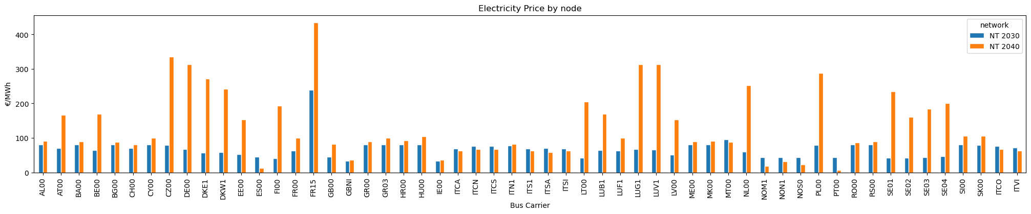
With this, we can extract electricity prices in the system across NT planning years. In line with the Market Model, we will aggregate the outputs using an average (weighting="time").

Note that you can easily choose if you want to calculate the price weighted by load instead by selecting weighting='load'.

prices = sc.prices(bus_carrier="AC", weighting="time").unstack("network")
prices.head(10)

network	NT 2030	NT 2040
name
AL00	80.854	91.300
AT00	70.461	167.147
BA00	80.475	90.099
BE00	64.460	169.947
BG00	80.841	88.048
CH00	69.952	80.298
CY00	80.952	100.626
CZ00	78.640	335.594
DE00	66.885	312.534
DKE1	57.100	271.531

For easier readability, we can plot them:

prices.plot.bar(
    figsize=(25, 4),
    edgecolor="white",
    ylabel="€/MWh",
    xlabel="Bus Carrier",
    title="Electricity Price by node",
);

_images/4149f59b71c6bc16c979e3c50f130fca45bec15bacc783960ee0a7a86461baed.png

Note

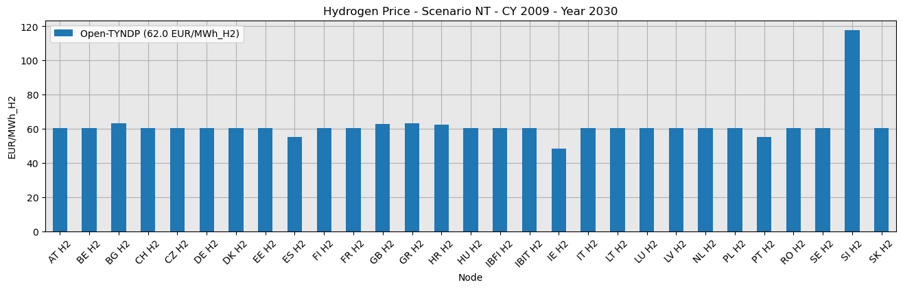
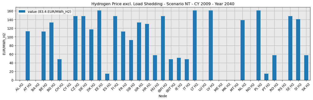
Please keep in mind that the methodology used to implement hydrogen and electricity market coupling slightly differs from the TYNDP 2024 approach. Unlike the Market Model, which assumes a fixed hydrogen fuel price for hydrogen-to-power generation, Open-TYNDP couples electricity and hydrogen markets by using endogenous hydrogen fuel price for them. This results in high price spikes induced by load shedding in the coupled market. This is especially visible in the NT 2040 outcomes. Detailed electricity price benchmarks excluding load shedding are available on Zenodo.

`PyPSA.Statistics` plotting APIs#

As we already introduced in a previous workshop, there is actually a quick way to explore the data with plots generated directly using the PyPSA.statistics module.

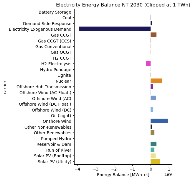
We can now explore the electricity energy balance for the NT 2030 network using this API directly.

fig, ax, _ = s2030.energy_balance.plot.bar(
    bus_carrier=["AC", "low voltage"],
    query=f"abs(value)>{clip * 1e6}",  # Values are in MWh
    height=6,
)

ax.set_title(f"Electricity Energy Balance {scenario} (Clipped at {clip} TWh)");

_images/fbddca2c217c42904fc54d0a14fc1ef823fb2796daf62041ea503e724216ad4a.png

…or we can even interactively explore the production of a specific technology in a specific country. For example January wind production in the Netherlands for NT 2030:

fig = s2030.energy_balance.iplot.area(
    facet_col="country",
    y="value",
    x="snapshot",
    carrier="wind",
    color="carrier",
    query="country == 'NL' and snapshot < '2009-02'",
    width=1200,
    height=500,
    title="Wind Production Netherlands NT 2030, January",
)

fig.update_layout(yaxis_title="Wind Production [MWh_el]")

As you can see, in January the Netherland’s wind mix is largely dominated by Offshore Wind production.

And of course NetworkCollections also work with PyPSA.statistics quick plotting API. So we can have a look at the previous price plot but using statistics plotting directly:

fig = sc.prices.iplot.bar(
    bus_carrier=["AC"],
    x="name",
    y="value",
    color="network",
    stacked=True,
    width=1200,
    height=500,
    nice_names=False,
    title="Electricity Price by node",
)

fig.update_layout(yaxis_title="Prices [EUR/MWh]")

Task 2: Grow comfortable with `PyPSA.statistics`#

Familiarize yourself with the statistics module (again) and explore the latest outcomes of Open-TYNDP using the different methods and plots introduced today.

Hint: You can also refer to the introduction above for more information on the different methods and parameters of PyPSA.statistics.

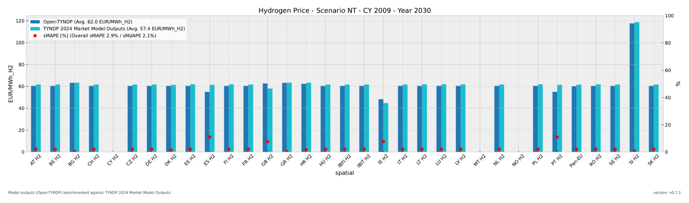
Task 3: Reproduce Benchmarks#

(a) If you feel comfortable using PyPSA.statistics, you can try to reproduce the Open-TYNDP outcomes from the following example of our latest benchmarking figures.

Try it without looking at the previous example first.

show_benchmarks(
    "benchmark_hydrogen_price_cy2009",
    [2030],
    "data/results-0.7.1/NT-cy2009-20260520/benchmarks/tyndp-2024/graphics_s_all___all_years/by_bus",
)

_images/2747adc8c27f7835bb95b4fdde13a3533262e654540e63faae4fc19e21bb6847.png

(b) Optional: Try to exclude load shedding from the hydrogen price in 2040.

Task 4 (Advanced): Inspect Outputs#

(a) Can you verify the total amount of wind generated on Danish Offshore Hubs in 2040 at 43.55 TWh?

Hint: The Offshore Hub bus carrier is AC_OH. Remember to include the Bornholm Energy Island bus called BEIOH01.

(b) Can you verify that Germany is the largest net annual importer of H2 in 2040?

Hint: Look for carrier="H2 pipeline|import" in the energy balance. Remember that you can group by bus or country.

(c) Can you investigate the correlation between electricity mix and H2 production in Germany for the first week of June in 2040? What can we notice?

Cost-Benefit Analysis#

Now that we’ve explored the Scenario Building (SB) results, let’s learn how to run Cost-Benefit Analysis (CBA)!

Clone the Open-TYNDP repository#

First, navigate into the data/ folder:

os.chdir("data/")
print("Directory changed to:", os.getcwd())

Directory changed to: /home/runner/work/open-tyndp-workshops/open-tyndp-workshops/open-tyndp-workshops/data

Clone the Open-TYNDP repository directly:

%%capture
if os.path.basename(os.getcwd()) == "data" and not os.path.exists("open-tyndp"):
    ! git clone https://github.com/open-energy-transition/open-tyndp.git

# Check open-tyndp was cloned successfully
if os.path.exists("open-tyndp"):
    print("Successfully cloned Open-TYNDP repository into local data folder!")

Successfully cloned Open-TYNDP repository into local data folder!

Now, navigate into the the open-tyndp directory:

os.chdir("open-tyndp/")
print("Directory changed to:", os.getcwd())

Directory changed to: /home/runner/work/open-tyndp-workshops/open-tyndp-workshops/open-tyndp-workshops/data/open-tyndp

Workflow management using `Snakemake` and `pixi`#

~15 minutes

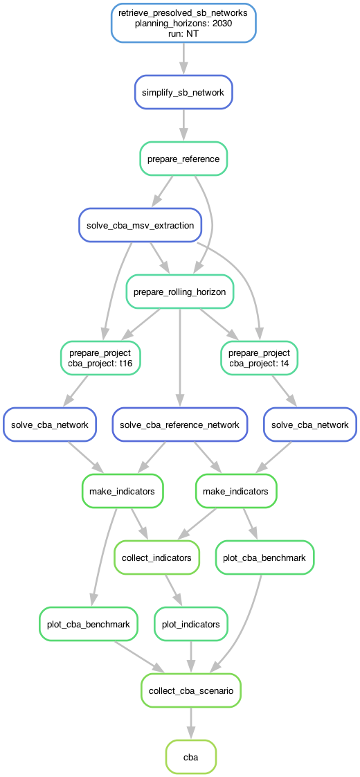
The Open-TYNDP CBA workflow involves many interconnected steps: from retrieving the SB network, to preparing the reference and project networks, to optimizing the networks, to calculating indicators.

To manage this complexity, Open-TYNDP uses two complementary tools:

Snakemake - A workflow management system that automatically figures out which analysis steps to run and in what order
pixi - A package manager that simplifies environment setup and provides easy-to-use shortcuts for running workflows

The combination of Snakemake and pixi allow Open-TYNDP to run with the flexibility to easily change configurations and run different scenarios.

Reminder: `Snakemake`#

The Snakemake workflow management system is a tool to create reproducible and scalable data analyses. Workflows are described via a human readable, Python based language. They can be seamlessly scaled to server, cluster, grid, and cloud environments, without the need to modify the workflow definition.

Snakemake follows the GNU Make paradigm: workflows are defined in terms of so-called rules that specify how to create a set of output files from a set of input files. Dependencies between the rules are determined automatically, creating a DAG (directed acyclic graph) of jobs that can be automatically parallelized.

Why does Open-TYNDP use Snakemake?

Running the full TYNDP analysis involves many steps that depend on each other.

Snakemake can automatically:

Determine which steps need to run based on what files already exist
Figure out the correct order to run them
Skip steps that don’t need to be re-run
Can run independent steps in parallel to save time

Note

Snakemake documentation: https://snakemake.readthedocs.io/

Snakemake introduction from Open-TYNDP Workshop 2

Using `snakemake`#

Snakemake workflows can be triggered in different ways:

By target file: specify the final output you want (using results/my_output.nc as an example output file name)
```
snakemake -call results/my_output.nc
```
By rule name: call a specific step in the workflow (using build_data as an example rule/step name)
```
snakemake -call build_data
```
NOTE: You cannot call a rule that includes a wildcard without specifying what the wildcard should be filled with. Otherwise, Snakemake will not know what to propagate back.
By entire workflow: Use the common rule all to execute the entire workflow. It takes the final workflow output as its input and thus requires all previous dependent rules to be run as well
```
snakemake -call all
```

The dry-run flag (`-n`)#

A very important feature is the -n flag which executes a dry-run. It is recommended to always first execute a dry-run before the actual execution of a workflow. This simply prints out the DAG of the workflow to investigate without actually executing it.

! snakemake -call -n

Introducing: `pixi`#

pixi is a cross-platform, multi-language package management and workflow tool. It is built on the foundation of the conda ecosystem.

Why does Open-TYNDP use pixi?

pixi serves two important roles in the Open-TYNDP project:

1. Environment Management
pixi automatically installs all the required Python packages and their correct versions, similar to conda but faster and more reliable. Pixi helps us not have to worry about package conflicts or missing dependencies.

2. Simplified Commands
pixi also allows us to create shortcuts for long snakemake commands.

You can see the full Snakemake commands that pixi runs by looking in the pixi.toml file in the Open-TYNDP repository. For example, we have defined a shortcut for running the full CBA workflow, called tyndp-cba:

display_code_lines("pixi.toml", "toml", 200, 202)

tyndp-cba = """
    snakemake -call cba --configfile config/config.tyndp.yaml
"""

Note

pixi documentation: https://pixi.prefix.dev/latest/.

Using `pixi`#

Without pixi (raw Snakemake), you would run this command to run the full CBA workflow:

snakemake -call cba --configfile config/config.tyndp.yaml

Using pixi, you just need to run:

pixi run tyndp-cba

For the remainder of this notebook, we will use pixi commands.

Installing Open-TYNDP#

# Uncomment the next line for running this notebook on Colab
# !wget -qO- https://pixi.sh/install.sh | sh

Note

If pixi was installed successfully but your shell still can’t find it, you may need to add it to your PATH manually. Use the following command to do so.

os.environ["PATH"] = os.path.expanduser("~/.pixi/bin") + ":" + os.environ["PATH"]

Use pixi to install the open-tyndp environment:

! pixi install -e open-tyndp

/bin/bash: line 1: pixi: command not found

Coupled vs decoupled SB-CBA workflow#

Before diving into the workflow, it helps to understand that there are two ways to run the CBA: (i) starting from scratch running first the SB, or (ii)using pre-solved networks we’ve already uploaded. The second option is much faster.

Coupled	Decoupled

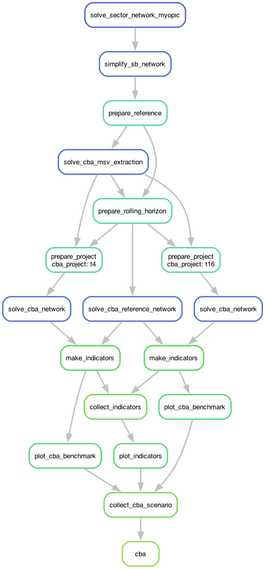
The two diagrams above illustrate the two different ways to run the CBA workflow:

Coupled Workflow (left):

Starts from scratch with the Scenario Building optimization
First solves the Scenario Building network (the solve_sector_network_myopic step)
Then continues on to perform the Cost-Benefit Analysis
Each CBA project goes through: prepare project -> optimize project and reference networks -> calculate indicators

Note: There are many rules (100+) that exist before solve_sector_network_myopic, but they are not included here for the diagram to be legible. With these diagrams, we mainly want to highlight the handoff between the SB process and the CBA process within the Open-TYNDP workflow.

Note: For each additional project you evaluate, the workflow adds more parallel branches. The diagram shows 2 projects just for illustrative purposes.

Decoupled Workflow (right):

Starts from pre-solved SB networks that we download from our releases
Skips all the Scenario Building steps – begins directly at the retrieve stage
The rest of the workflow is identical to the coupled approach
Much faster because we can skip the Scenario Building steps (including the optimization)

Coupled SB->CBA workflow#

~20 minutes

Configuration Options

The Open-TYNDP workflow’s settings are housed in config/config.tyndp.yaml. Feel free to open the file to explore the full extent of configuration settings we have available.

One key parameter that affects both the SB and CBA processes is the run name, which sets what scenario(s) to run - for example, the parameter can be changed to “NT” to run just the NT scenario:

display_code_lines("config/config.tyndp.yaml", "yaml", 6, 8)

run:
  prefix: "tyndp"
  name: "all"

Some CBA-specific key parameters are:

display_code_lines("config/config.tyndp.yaml", "yaml", 411, 432)

cba:
  hurdle_costs: 0.01 # Transmission line marginal cost
  co2_societal_cost: # euros/t; 2024 CBA Implementation Guidelines, p. 68
    2030:
      low: 126
      central: 238
      high: 315
    2040:
      low: 339
      central: 628
      high: 662
  planning_horizons:
  - 2030
  - 2040
  cba_scenario_input:
    use_presolved: false
    sb_version: latest # use 'latest' or a supported version from data/versions.csv for pre-solved SB network input in CBA; only applies if use_presolved is true
  methods:
  - toot
  - pint
  projects:
  - t1-t35

You can modify the config settings within Open-TYNDP in two ways:

Edit the config file directly
Override via command line – For example, by adding the following to your command: --config 'run={"name":"NT"}' 'cba={"planning_horizons":[2030]}'

Tip

In practice, editing the YAML configuration files directly in a text editor or IDE is much easier than using command-line overrides. We’re using command-line options in this notebook for demonstration purposes, but for real life, we recommend modifying the config files directly!

Triggering a complete CBA run

As hinted earlier, the command pixi run tyndp-cba executes the complete CBA workflow:

Takes a solved Scenario Building network (either from scratch or using pre-solved network)
Prepares the CBA reference and project networks, for the specified project(s)
Evaluates each specified project using TOOT or PINT methodology
Calculates indicators (B1-B4)

First, let’s check what running the full workflow could look like by doing a dry-run of pixi run tyndp-cba:

! pixi run tyndp-cba -n

/bin/bash: line 1: pixi: command not found

We can specify the specific scenario (e.g, NT), the project (e.g., t4), and planning horizon (e.g., 2030) we want to run directly in the command line.

! pixi run tyndp-cba --config 'run={"name":"NT"}' 'cba={"planning_horizons":[2030],"projects":["t4"]}' -n

/bin/bash: line 1: pixi: command not found

Notice how the count of steps changed when we specified a single run, project, and horizon.

Comparatively, the default settings in Open-TYNDP is set to run:

NT, DE, GA, and all climate year variations of these scenarios
two planning horizons (2030 and 2040)
5 CBA projects (t4, t16, t28, t33, t35)

Thus, running the full default CBA workflow will trigger many, many more steps, since the DAG has to be expanded for all scenarios, planning horizons, and projects.

Checkpoints#

You may notice above that the number of rules is actually quite low.

There is a checkpoint in the workflow, called clean_projects, that first checks how many projects are being asked to run before building out the full DAG. It tells the workflow which CBA projects exist, which project IDs to run, and which method applies (TOOT/PINT).

Before the clean_projects step runs, Snakemake does not know the full list of project jobs it needs to create. The step downloads and cleans the external CBA project database, tells the workflow the full list of projects available, which projects the user wants to evaluate, and how each should be evaluated. After clean_projects finishes, Snakemake can read the cleaned CSV and expand the DAG into concrete jobs.

Thus, what we should do first here is run the workflow just up until the checkpoint, then only after that can we run the full workflow again – in which case, the DAG would show the actual number of jobs that would be run.

! pixi run tyndp-checkpoint --config 'run={"name":"NT"}' 'cba={"planning_horizons":[2030],"projects":["t4"]}'

/bin/bash: line 1: pixi: command not found

Now that the checkpoint is complete, we can re-check the DAG of how many steps are needed to run the CBA workflow.

! pixi run tyndp-cba --config 'run={"name":"NT"}' 'cba={"planning_horizons":[2030],"projects":["t4"]}' -n

/bin/bash: line 1: pixi: command not found

Task 5: Configure the settings in config files#

So far, we’ve been setting the run settings via the command line. However, as we’ve mentioned, in real life it’s much easier to go into the config files and edit them directly. So let’s do that for the settings we’ve been running the CBA with so far:

NT run
2030 planning horizon
t4 project

Instructions:

Open config/scenarios.tyndp.yaml
Find the NT scenario definition (it’s the first one)
Modify the NT scenario so that it looks like this:

NT:
  tyndp_scenario: NT

  cba:
    planning_horizons: [2030]
    projects: ["t4"]

Save the file
Open config/config.tyndp.yaml in a text editor
Set run: name: to "NT". The top section of your file should look like:

run:
  prefix: "tyndp"
  name: "NT"

Save the file
Come back to this notebook to run the checkpoint: ! pixi run tyndp-checkpoint
Then run the dry-run: ! pixi run tyndp-cba -n

You should see the same number of steps as when we ran ! pixi run tyndp-cba --config 'run={"name":"NT"}' 'cba={"planning_horizons":[2030],"projects":["t4"]}' -n above.

Now you can run the CBA workflow without needing to specify configuration overrides on the command line!

Run different and multiple climate years#

~15 minutes

Understanding Climate Years

Energy system performance varies significantly with weather conditions - wind and solar availability change year to year, as do heating and cooling demands. To account for this variability, Open-TYNDP can evaluate scenarios using different historical climate years.

Climate year scenarios are defined in config/scenarios.tyndp.yaml. For example:

display_code_lines("config/scenarios.tyndp.yaml", "yaml", 210, 220)

NT-cy2008:
#  <<: *cba-common
  snapshots:
    start: "2008-01-01"
    end: "2009-01-01"

  atlite:
    default_cutout: europe-2008-sarah3-era5

  cba:
    sb_scenario: NT

The following climate year scenarios related to the NT scenario are already existing in the Open-TYNDP workflow:

NT-cy1995: NT scenario using 1995 weather data
NT-cy2008: NT scenario using 2008 weather data
NT-cy2009: NT scenario using 2009 weather data
NT-cyears: Runs all 3 NT scenarios: NT-cy1995, NT-cy2008, and NT-cy2009

The NY-cyears scenario acts somewhat as a collection scenario for the 3 climate years and is defined in config/scenarios.tyndp.yaml as well:

display_code_lines("config/scenarios.tyndp.yaml", "yaml", 314, 316)

NT-cyears:
  cba:
    scenarios: [NT-cy2009, NT-cy2008, NT-cy1995]

How can we run the CBA workflow for a different climate year? First, we again need to run up to the checkpoint for the different climate years:

! pixi run tyndp-checkpoint --config 'run={"name":["NT-cy2008", "NT-cy2009", "NT-cy1995"]}' 'cba={"planning_horizons":[2030],"projects":["t4"]}'

/bin/bash: line 1: pixi: command not found

Now, we can run for just another climate year, such as the 1995 climate year for the NT scenario (NT-cy1995):

! pixi run tyndp-cba --config 'run={"name":"NT-cy1995"}' 'cba={"planning_horizons":[2030],"projects":["t4"]}' -n

/bin/bash: line 1: pixi: command not found

Or, we can run all climate years (1995, 2008, and 2009), which falls under the NT-cyears scenario:

! pixi run tyndp-cba --config 'run={"name":"NT-cyears"}' 'cba={"planning_horizons":[2030],"projects":["t4"]}' -n

/bin/bash: line 1: pixi: command not found

Notice how the total count of steps is much higher (especially for CBA-specific steps such as make_indicators and weather-dependent steps such as build_renewable_profiles_pecd) when multiple climate years are run.

Task 6: Create your own climate year scenario#

Create your own custom climate year scenario by modifying config/scenarios.tyndp.yaml:

Instructions:

Open config/scenarios.tyndp.yaml .
Find an existing climate year definition (e.g., NT-cy2008).
Copy the entire section and give it a new name (e.g., NT-workshop or anything you like).
Modify the parameters as desired (e.g., set the snapshots to the climate year you’re interested in - note that we’re limited to 1995, 2008, and 2009).
Add CBA configuration to your custom scenario (similar to what you did in Task 5):

    cba:
      sb_scenario: NT
      planning_horizons: [2030]
      projects: ["t4"]

In the end, the full custom scenario should look something like this:

    NT-workshop:
    #  <<: *cba-common
      snapshots:
        start: "2008-01-01"
        end: "2009-01-01"

      atlite:
        default_cutout: europe-2008-sarah3-era5

      cba:
        sb_scenario: NT
        planning_horizons: [2030]
        projects: ["t4"]

Save the config/scenarios.tyndp.yaml file,
Update config/config.tyndp.yaml to set run: name: to "NT-workshop" (or your custom scenario name). Save file.

By configuring the CBA settings in your scenario file, you can now run it with just: pixi run tyndp-cba -n (but first, remember to run the checkpoint).

Warning

The weather data availability is limited. Currently, only climate years 1995, 2008, and 2009 are available in the pre-built PECD (Pan-European Climate Database) that Open-TYNDP uses. The data is reduced to minimise retrieval requirements.

Decoupled SB->CBA workflow#

~10 minutes

You may have noticed by now that when running the coupled SB and CBA workflow, even when running the CBA for just 1 project, 1 planning horizon, and 1 scenario, this could trigger 100+ steps to be run.

Within Open-TYNDP, we have the flexibility to retrieve a pre-solved SB network (uploaded to Zenodo and Google Cloud as part of the project releases) and use this pre-solved SB network

This can be easily done by setting the cba.use_presolved setting to true. By default, this downloads and uses the latest release we have (at the time of this workshop, that is v0.7.1).

! pixi run tyndp-cba --config 'run={"name":["NT"]}' 'cba={"cba_scenario_input":{"use_presolved":true,"sb_version":"latest"},"planning_horizons":[2030],"projects":["t4"]}' -n

/bin/bash: line 1: pixi: command not found

Note how the number of steps has decreased down from over 100 to just ~37, and we see some new steps not previously seen before, such as retrieve_presolved_sb_networks.

You can also specify a different version to retrieve from - for example, the previous release (0.6.1):

! pixi run tyndp-cba --config 'run={"name":["NT"]}' 'cba={"cba_scenario_input":{"use_presolved":true,"sb_version":"0.6.1"},"planning_horizons":[2030],"projects":["t4"]}' -n

/bin/bash: line 1: pixi: command not found

At the moment, Open-TYNDP has only run the SB process on the NT scenario, so we can only use pre-solved networks for the NT scenario (meaning, you cannot set use_presolved to true and change the run name to “DE” for example).

Task 7 (optional): Perform a complete (decoupled) Cost-Benefit Analysis#

Optional Exercise: Run a Complete CBA

If you have time and want to see the full workflow in action, you can run a complete CBA evaluation using a pre-solved network:

First, navigate into a specific branch called workshop-4-cba in git:

! git checkout workshop-4-cba

We created this branch to allow for a successful lower-resolution optimization within feasible time. Note, that in order for the entire workflow to pass, you might need to run this task locally as it can run into the free computational resources limit on Google Colab.

The only changes made to this branch are changes to config.tyndp.yaml:

retrieve data from Google Cloud (instead of Zenodo)
remove hydro-reservoir state of charge constraint
allow load sinks for CO2 sequestration

The first adjustment is just to speed up retrieval times, while the last two adjustments are needed mainly to alleviate constraint conflicts from the lower temporal resolution of used in the optimization for this workshop (otherwise, we normally solve at 1H resolution, which takes too long for such an exercise). The changes made can also easily be seen in the Github Pull Request associated with the branch: open-energy-transition/open-tyndp#changes.

After checking out the branch, you can run the following command:

! pixi run tyndp-cba --config 'run={"name":"NT"}' 'data_config=tyndp' 'cba={"planning_horizons":[2030],"cba_scenario_input":{"use_presolved":true,"sb_version":"latest"},"projects":["t16"],"msv_extraction":{"resolution":"24H"}}'

What this command does:

Downloads the pre-solved NT 2030 network
Reduces the resolution of the MSV down to 24H (necessary for faster solve in this example)
Evaluates project t4 by optimizing the project network (with 1 week rolling horizon)
Calculates all CBA indicators
Produces final results in results/tyndp/NT/cba/

Time requirement: This could take approximately 15-20 minutes to complete, depending on your computer’s performance. So this would be a good task to start right before going on a coffee break!

If you completed Task 5 or 6, your config file will have been modified. Run the cell below to reset it before switching branches:

! git restore config/config.tyndp.yaml

Checkout to the workshop-specific branch:

! git checkout workshop-4-cba

branch 'workshop-4-cba' set up to track 'origin/workshop-4-cba'.
Switched to a new branch 'workshop-4-cba'

Now, you can trigger the run of the complete CBA workflow (using a pre-solved SB network):

! pixi run tyndp-cba --config 'run={"name":"NT"}' 'cba={"planning_horizons":[2030],"cba_scenario_input":{"use_presolved":true,"sb_version":"latest"},"projects":["t4"],"msv_extraction":{"resolution":"24H"}}'

/bin/bash: line 1: pixi: command not found

Optional: Modifying assumptions in Open-TYNDP#

A key advantage of open-source energy modelling is the ability to adjust assumptions and immediately see how results respond. Open-TYNDP offers several ways to do this, ranging from simple data updates to custom constraints:

Method	What it does	Where
Input data	Replace or update raw input files	`data/` folder
Custom assumptions	Override cost & technology parameters for specific technologies and planning horizons	`data/custom_cost.csv`
Adjustments	Apply scaling factors or absolute overrides to specific components directly in the scenario config	`config/scenarios.tyndp.yaml`
Custom constraints	Add or modify optimisation constraints beyond what the config exposes	`scripts/solve_network.py`

Methods are ordered from simplest to most advanced — for most use cases, input data or custom assumptions are the right starting point.

Solutions#

Task 2: Reproduce benchmarks#

# (a) Try to reproduce the Open-TYNDP outcomes from the hydrogen prices example above from our latest [benchmarking figures](https://zenodo.org/records/20303009).

show_benchmarks(
    "benchmark_hydrogen_price_cy2009",
    [2030],
    "../results-0.7.1/NT-cy2009-20260520/benchmarks/tyndp-2024/graphics_s_all___all_years/by_bus",
)

Task 3: Investigate outputs#

Show code cell content

Hide code cell content

# (b) Can you verify that Germany is the largest *net annual importer of H2* in 2040?
(
    s2040.energy_balance(
        bus_carrier="H2",
        carrier="H2 pipeline|import",
        aggregate_across_components=True,
        groupby=["carrier", "country"],
    )
    .div(1e6)  # TWh
    .droplevel("carrier")
    .groupby("country")
    .sum()
    .sort_values(ascending=False)
    .to_frame("H2 Import (+), H2 Export (-) [TWh]")
    .head()
    .style.format("{:,.2f}")  # Make style a bit prettier
)

	H2 Import (+), H2 Export (-) [TWh]
country
DE	314.89
IT	95.79
FR	91.15
PL	89.05
BE	65.32

We can observe for night of the 5th of June, that wind production drops along with solar electricity production resulting in no hydrogen production via electrolysis for that time. Instead, German hydrogen demand is met via H2 pipeline imports as well as from Cavern Storages and blue Hydrogen production. Pumped hydro, battery storage and electricity imports are utilized to support electricity production in the same period to meet the remaining exogenous electricity demand.

Task 5: Modify Configuration Files Directly#

After modifying config/scenarios.tyndp.yaml so that the NT scenario is:

NT:
  tyndp_scenario: NT

  cba:
    planning_horizons: [2030]
    projects: ["t4"]

Task 6: Create a Custom Climate Year Scenario#

After creating your custom scenario in config/scenarios.tyndp.yaml (e.g., named “NT-workshop”):

Notebook clean up#

# Only clean up data when running in CI environment
if os.getenv("CI"):
    rm_dir = "data/results-0.7.1"
    print(
        f"CI environment detected. Cleaning up notebook data by removing '{rm_dir}' and '{rm_dir}.zip'."
    )
    shutil.rmtree(rm_dir, ignore_errors=True)
    Path(f"{rm_dir}.zip").unlink(missing_ok=True)
else:
    print("Skipping cleanup (not in CI environment).")

CI environment detected. Cleaning up notebook data by removing 'data/results-0.7.1' and 'data/results-0.7.1.zip'.

Workshop 4: Open-TYNDP Outcomes and CBA Workflows

Contents

Workshop 4: Open-TYNDP Outcomes and CBA Workflows#

Scenario Building#

Reminder: Extracting insights from the network#

Interactive Exploration with PyPSA-Explorer#

Reminder: Using the Dashboard#

For Local Users#

For Google Colab Users#

Task 1: Navigate PyPSA-Explorer#

Explore NT outcomes using the PyPSA.statistics module#

Reminder: Extracting insights from a network#

Compare results with PyPSA.NetworkCollections#

PyPSA.Statistics plotting APIs#

Task 2: Grow comfortable with PyPSA.statistics#

Task 3: Reproduce Benchmarks#

Task 4 (Advanced): Inspect Outputs#

Cost-Benefit Analysis#

Clone the Open-TYNDP repository#

Workflow management using Snakemake and pixi#

Reminder: Snakemake#

Using snakemake#

The dry-run flag (-n)#

Introducing: pixi#

Using pixi#

Installing Open-TYNDP#

Coupled vs decoupled SB-CBA workflow#

Coupled SB->CBA workflow#

Checkpoints#

Task 5: Configure the settings in config files#

Run different and multiple climate years#

Task 6: Create your own climate year scenario#

Decoupled SB->CBA workflow#

Task 7 (optional): Perform a complete (decoupled) Cost-Benefit Analysis#

Optional: Modifying assumptions in Open-TYNDP#

Solutions#

Task 2: Reproduce benchmarks#

Task 3: Investigate outputs#

Task 5: Modify Configuration Files Directly#

Task 6: Create a Custom Climate Year Scenario#

Notebook clean up#

Task 1: Navigate `PyPSA-Explorer`#

Explore NT outcomes using the `PyPSA.statistics` module#

Compare results with `PyPSA.NetworkCollections`#

`PyPSA.Statistics` plotting APIs#

Task 2: Grow comfortable with `PyPSA.statistics`#

Workflow management using `Snakemake` and `pixi`#

Reminder: `Snakemake`#

Using `snakemake`#

The dry-run flag (`-n`)#

Introducing: `pixi`#

Using `pixi`#