Detection model
The task, seen at 10 m
Everything about this model follows from one number: a Sentinel-2 pixel is 10 by 10 metres. A large array spans tens of pixels and has a shape the model can outline. A domestic array does not even fill one pixel; its only trace is a slight change in that pixel's colour, mixed with whatever roof surrounds it.
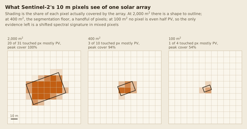
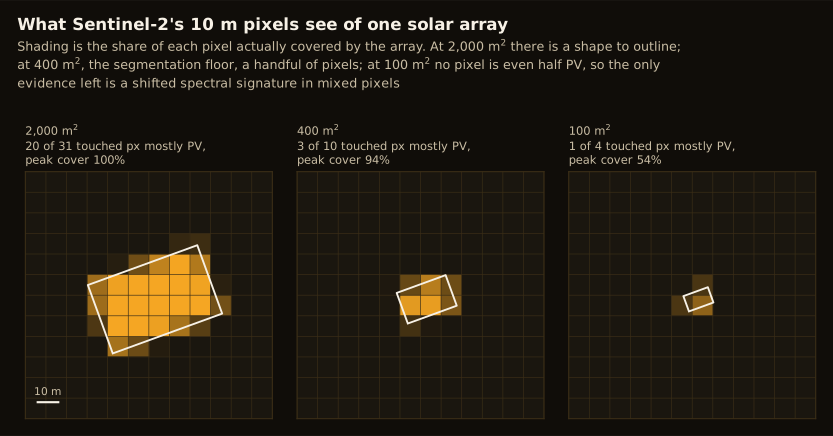
That is why the project runs two detectors in two different domains, split at 400 m2:
- Spatial domain, this page. Above the floor there is an outline to find, so a
segmentation model labels each pixel PV or not and
postprocessturns the labelled pixels into candidate polygons. - Spectral domain, the rooftop classifier. Below the floor there is no outline, only mixed pixels, so the question changes from "where are the panel edges" to "does this building's spectral signature look like it carries PV". That is a per-building classification, not a segmentation.
The floor is enforced in training, not just observed: MIN_PV_AREA burns everything
below it into the training mask as ignore, so the segmentation model receives no
gradient there at all (see Positive threshold below).
The model
terramind_v1_tiny, the open TerraMind geospatial foundation model from IBM and ESA,
fine-tuned as a semantic segmentation task through TerraTorch and Lightning. Tiny is not a
compromise for its own sake: it fits a 6 GB GTX 1060, which keeps the whole project
reproducible on hardware a university lab already owns.
TerraMind is a plain vision transformer, so a UNet decoder needs a feature pyramid built
for it. The neck stack is SelectIndices into ReshapeTokensToImage into
LearnedInterpolateToPyramidal. Checkpoints monitor validation mIoU (mean Intersection over Union).
Bands. Local composites carry 10 bands, B02 through B12 minus the two 60 m atmospheric
bands B01 and B09. TerraMind's pretrained Sentinel-2 L2A patch embedding expects 12, so
configs/terramind_pv.yaml passes backbone_bands: {S2L2A: [...]} and TerraTorch subsets
the patch embedding to exactly those 10. The pretrained weights for the bands in use are
kept; the rest are dropped rather than zero-padded.
Positive threshold. MIN_PV_AREA in chips.py sets the smallest labelled array that
is burned as a positive. Arrays below it are burned as ignore = -1, not as negatives, so
the loss never learns that a small real array is background. Changing it means rebuilding
chips and retraining.
What it recovers
Per-installation recall at threshold 0.3, checkpoint v2_combined/terramind-pv-epoch=39,
trained on 3,189 German chips plus 274 Punjabi chips:
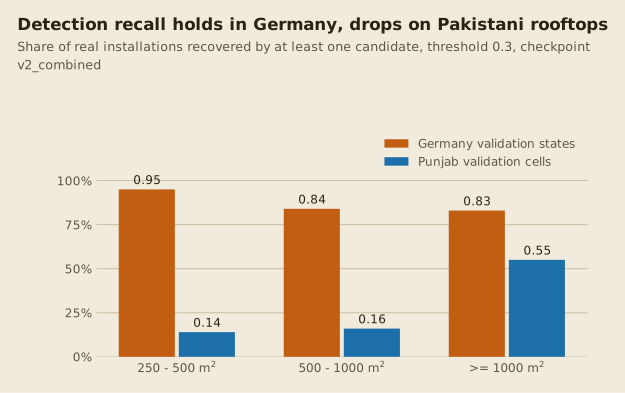
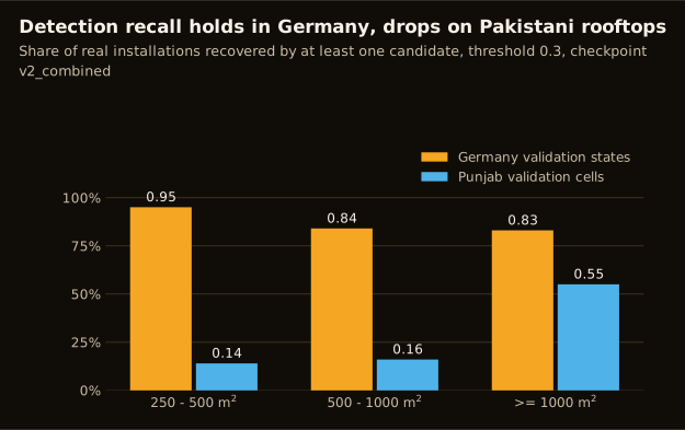
Pixel IoU and F1 are 0.51 and 0.68 on Germany, 0.29 and 0.45 on Punjab.
The Punjab column is much weaker than Germany's, and it is also three times what the Germany-only model achieved on the same cells (0.18 at or above 1,000 m2). In-domain chips are the single biggest lever found so far, which is the empirical case for the mapping flywheel.
The residual Punjab misses look imagery-limited rather than model-limited. The model outputs near-zero probability on them even at threshold 0.05, and oversampling Punjab four times did not move it. Smog-season composites, mixed pixels and label noise in the Pakistani OpenStreetMap extract are the plausible causes.
A high false-positive rate is expected and accepted on this path. Candidates are validated by people against high-resolution imagery, so a false positive costs seconds and a miss costs everything.
From composite to candidate, on real installations
The whole spatial-domain pipeline is three steps, and all three are visible in one image: read the dry-season composite, predict a per-pixel probability, then threshold at 0.3 and polygonize whatever remains. These are four real Pakistani installations from the national inference run behind the published atlas, one per size bracket:
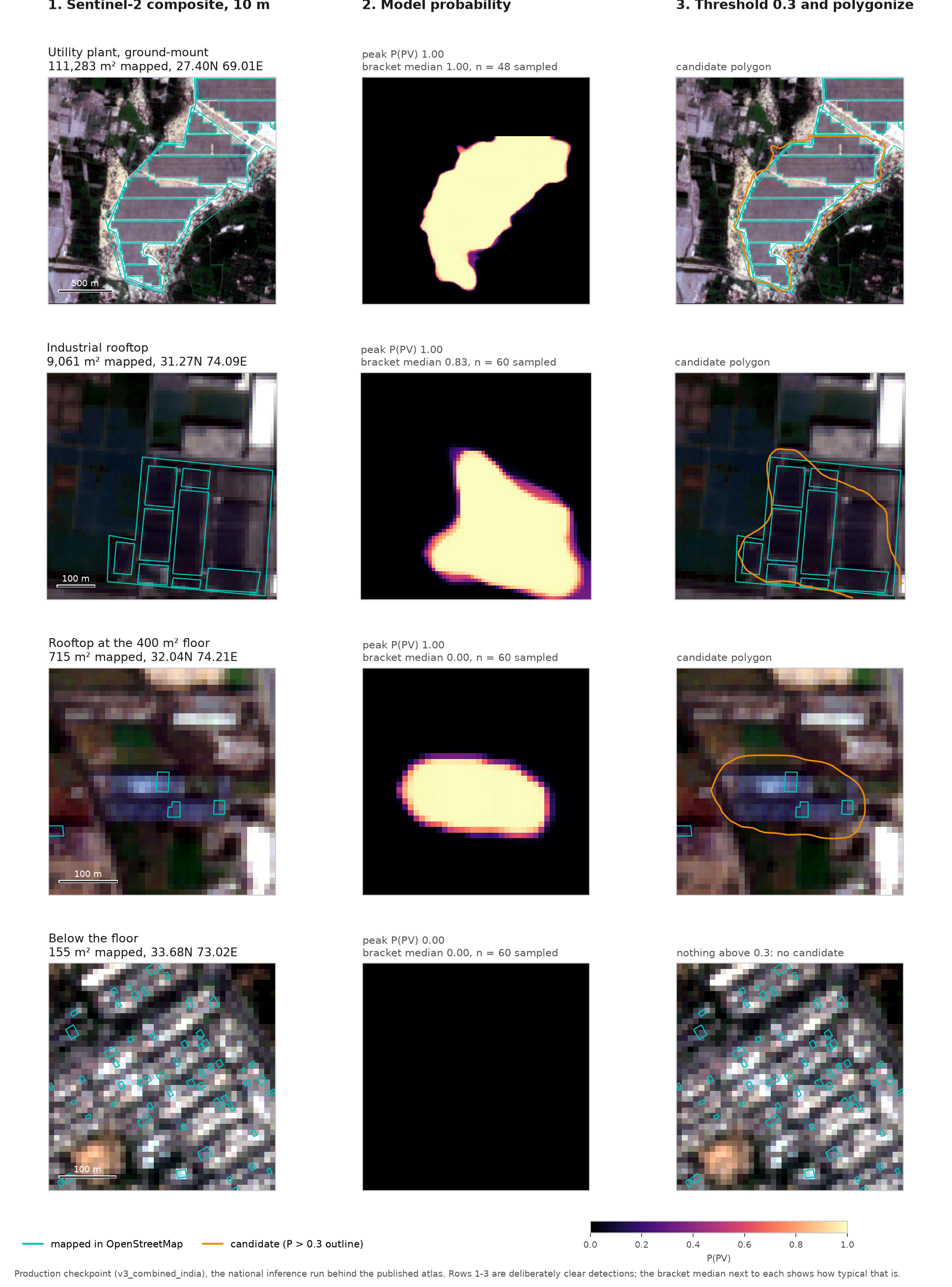
Reading it row by row:
- A utility-scale plant is unmissable. At 111,283 m2 the plant is a thousand pixels; the model saturates at probability 1.0 and the candidate polygon traces the real perimeter. This is why ground-mount capacity rests on segmentation alone.
- A large industrial rooftop works nearly as well (peak 1.0; the median over 60
sampled installations in the 2,000 to 10,000 m2 bracket is 0.83). The
candidate polygon is coarser than the mapped outlines, which is expected: the human
mapper draws each roof section, the model draws the blob of confident pixels, and
postprocesslater swaps in the mapped OSM geometry where one matches. - At the 400 m2 floor detection becomes a coin toss weighted against the model. The 715 m2 example is a clean hit, chosen to show what a hit looks like, but the honest number sits next to it: the median peak probability across its sampled bracket is 0.0. Most installations this size produce nothing.
- Below the floor there is nothing to threshold. The last row is a dense residential
block with dozens of mapped installations; the probability panel is uniformly black.
This is not a tuning problem: the model was never trained on arrays this small (they
are burned as
ignore), and no threshold recovers a probability that was never raised. Everything below this line belongs to the rooftop classifier, which asks the spectral question instead.
The first three rows are deliberately the clearest detections in their brackets, because the figure illustrates the mechanism; the bracket medians printed on the figure keep the recall picture honest, and the recall chart above is the systematic measurement.
Two invariants that must not regress
Naive sliding-window inference produced a regular grid of false positives at the window spacing. Both causes are fixed, and both fixes are load-bearing.
Training centre bias, the dominant cause. Positive chips are jittered by up to 900 m
in chips.py::sample_chip_centers, so the installation lands anywhere in the frame. Without
the jitter the model learns that PV is in the middle and fires once per window at
inference. The diagnostic is a spike in nearest-neighbour distance between detections at
exactly the window stride: 60 percent of detections were one stride apart before the fix,
about 7 percent after.
Window seams. infer.py overlap-adds windows with a 2D Hann taper into one seamless
raster per cell, and uses a stride that is deliberately not a multiple of the 16 px
transformer patch size (currently 104) so patch-edge effects decorrelate between
neighbours.
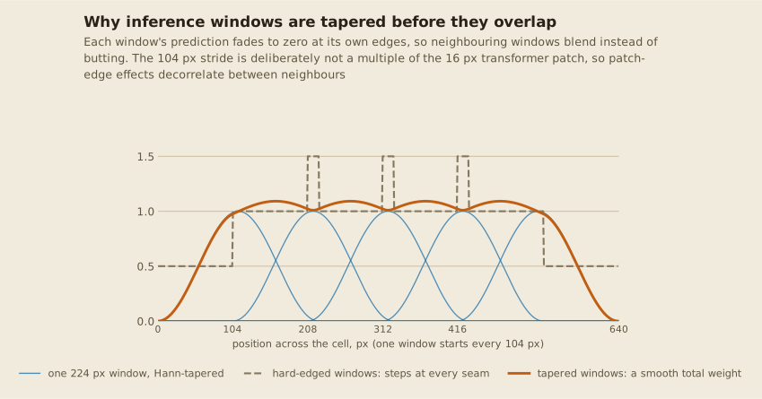
The picture is the whole argument: a hard-edged window contributes with full weight right up to its boundary and then not at all, so any disagreement between neighbouring windows becomes a visible seam, and seams at a fixed spacing become a fake grid of candidate edges. The taper makes every prediction fade to zero at its own edge, so neighbours blend where they overlap and no position in the final raster is dominated by a window boundary.
Imagery
Sentinel-2 L2A dry-season composites, the median of roughly the twelve least-cloudy scenes
per 0.1 degree cell. Where a sibling project already downloaded per-MGRS-tile composites
they are reused; everywhere else earthpv compose builds them on demand from Microsoft
Planetary Computer STAC, with Earth Search on AWS Open Data as a fallback with a different
failure domain.
Compose only touches building-populated cells, prioritized by building density, because rooftop PV needs roofs. That reduces "all of Pakistan" from an intractable raster job to roughly 4,470 cells. It is network-bound at about one to two minutes per cell, and resumable.
Candidates and ranking
postprocess.py thresholds and polygonizes the probability raster, then joins each
candidate to a building footprint set in the candidates' local UTM zone, recording
building_overlap_frac and building_dist_m. Those feed a building_prior and
rank_score = confidence x (0.5 + 0.5 x prior). This is a summary; the full walk-through
of the join, the placement rule and what each product does with it is
Segmentation & the building map.
Footprints come from VIDA Open Buildings (Google and Microsoft combined), which is
imagery-derived and includes small unmapped structures, so "no building within 30 m"
becomes a usable false-positive signal. The Overture set of buildings above 500 m2
is the fallback. For a candidate set dominated by large arrays on already-mapped buildings, the two footprint sources produce almost identical results; VIDA's advantage appears as soon as MIN_PV_AREA
drops toward residential scale.
Configurations
| File | Purpose |
|---|---|
configs/terramind_pv.yaml |
production, 10-band segmentation |
configs/terramind_pv_fraction.yaml |
per-pixel PV coverage fraction regression |
configs/terramind_pv_fraction_pakistan.yaml |
fraction head retrained in domain |
configs/terramind_pv_seasonal.yaml |
20-band two-season stack (negative result) |
configs/terramind_pv_v3india.yaml |
Germany plus Pakistan plus India combined |