How it works

This page describes the pipeline as it runs today: two detectors, split by placement and calibration coverage rather than by size alone, combined into one evidence atlas. Workflow tells the human story of how a Sentinel-2 pixel becomes a verified OpenStreetMap feature. Architecture is the technical complement, covering what reads what, stage by stage, and what is optional alongside the default path. Methods links out to the deep-dive reference page for each stage. Comparison sets the resulting figure against every other public estimate of Pakistan's solar fleet.

Two things deliberately live elsewhere, so that this page stays a description of the working pipeline rather than a history of the project: Experiments is the record of everything that was tried, including the majority that did not ship.

Workflow

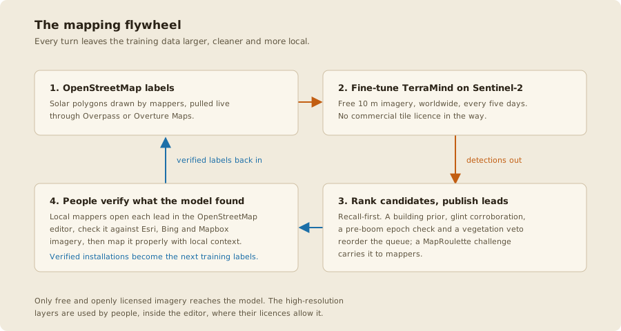
The technical novelty in EarthPV is not one model. It is a wheel that combines free low-resolution imagery, open foundation models, human mappers working inside OpenStreetMap with the high-resolution imagery they are already licensed to look at, and the local data a country already keeps. The model does three of its six stations and people do the other three; OpenStreetMap sits at the hub, because everything people map goes in there and comes back out as counted capacity and as training labels. Each turn leaves the map more complete, the models more local and the estimate better measured.

Why the loop exists

Two licences pull in opposite directions, and the loop is what resolves them.

Sentinel-2 is free, global, and reprocessed every five days, but at 10 m per pixel a typical rooftop array is four to twenty pixels. Esri, Bing and Mapbox imagery resolves individual panels, but their terms allow a person to trace from them inside the OpenStreetMap editor and do not allow a machine to be trained on them.

So the machine only ever reads Sentinel-2, and people only ever read the high-resolution layers. The model proposes; a mapper disposes; the disposal is recorded in OpenStreetMap as an ordinary, openly licensed feature; and that feature is legitimate training data for the next model. Nothing proprietary crosses into the model, and nothing the model produces is trusted until a person has looked at it.

The leads alone would turn the wheel for large arrays, which is how it started. Most of a country's rooftop solar is too small for any 10 m model to outline, and a number for it needs two things a lead cannot give: areas where every panel is mapped, to fit and check the small-installation estimate on, and whatever the country itself already counts, to set the result beside. Those are stations 4 and 5.

The six stations

1. Detect from space

earthpv infer runs the country's TerraMind checkpoint over every 0.1° cell of dry-season Sentinel-2 composites and writes one probability raster per cell. Below the 400 m² floor, where an array has no outline in 10 m pixels, a per-building classifier (roofclf) scores every roof and, where farm areas calibrate it, a pixel detector (groundclf) scores small arrays beside fields (two ways to see a panel). Building footprints come from VIDA Open Buildings, which is imagery-derived and therefore includes the small structures OpenStreetMap does not yet have.

2. Publish the evidence atlas and the leads

earthpv postprocess polygonizes each raster, attaches each candidate to a building footprint, and scores it. The pipeline is deliberately recall-first: false positives cost a mapper a few seconds, whereas a missed installation is invisible forever. Nothing is dropped by the default export. What the priors do is reorder the queue so mappers hit real installations first:

Signal	What it does	Direction
Building prior	overlap with, or distance to, a VIDA footprint	reorders
Glint corroboration	specular flashes consistent with one panel plane	boosts only
Pre-boom epoch check	high probability in 2021 imagery too, so probably not new PV	demotes
Vegetation veto	a crop cycle observed over the year, so not a panel	drops, into a separate clean file

earthpv export writes GeoParquet, GeoJSON and a MapRoulette challenge ordered by rank_score, and each country's atlas links its file of mapping leads: the candidates more than 100 m from any solar installation already in OpenStreetMap. The atlas itself publishes the best estimate with its 90% range and every gap as a gap: cells nobody imaged are hatched, an instrument that has not been calibrated reads "not measured" rather than zero, and the candidate calibration areas still to map are drawn on the map, a star on the one to start with.

3. Map the leads

Mappers open each lead in the OpenStreetMap editor, compare it against the high-resolution layers, and either map the installation properly or discard the lead. Local mappers add what no imagery shows: which industrial estate this is, whether the roof belongs to a factory or a school, whether the array is net-metered. Leads carry no completeness rule (Map the leads with JOSM).

4. Map calibration areas

A calibration area is a box, usually 1 to 3 km across, in which a mapper traces every visible panel down to the smallest rooftop unit (the protocol). New candidates are drawn at random across a country's building-density range rather than picked by hand, so the sample is not chosen for its solar. Complete areas are what the small-installation half is fitted and tested on: roofclf's leave-one-area-out skill, its coverage ratio and area recall per building size and density stratum, and the density band a figure is published in all come from them (Calibration quadrats). Pakistan has 30 in its fit. A country without any publishes large installations only, and its atlas says so.

5. Investigate local datasets

Every country keeps some count of its own solar: a register, the statistics office or energy ministry, a utility's net-metering list, a published study. Each one found is read for what it actually counts (registered or installed, AC or DC, rooftop or ground, above which size) and for its licence, then drawn beside the atlas in its Against official and published figures section, nationally and per province. None is treated as ground truth for the map, and none is used to score it. A register that is legally complete and geolocated goes further and becomes a calibration instrument: Germany's MaStR replaces calibration areas for its small-installation half and measures segmentation's precision, France's ODRE register measured the module constant at 0.150 kWp/m², and India's MNRE register puts ground-mounted Best at 0.73 of registered with a rank agreement of 0.97 over 19 states. Customs records give an import ceiling where a country has no domestic manufacturing.

6. Retrain the model and recalibrate

Newly mapped installations come back through the live Overpass pull (earthpv overpass-labels). earthpv chips cuts training windows around them and burns the label polygons into per-pixel masks, and earthpv train fine-tunes TerraMind-tiny on the country's own labels. The localized checkpoint ships only if it beats the general model on a held-out region (a tie goes to the local one); see Detection model. This is where the wheel first paid off: the label-driven compose in Punjab unlocked roughly 2,500 in-domain Pakistani positives, and adding them tripled large-array recall there against the Germany-only model.

Newly registered calibration areas refit roofclf and its coverage ratio, can widen the density band a figure is published in, and reviewed samples of the model's candidates re-derive its precision table. The next turn of station 1 starts from all of it.

An LLM assistant at every station

EarthPV is built and run with an LLM coding assistant, and the repository is written to be read by one: CLAUDE.md holds the pipeline's current state, its invariants and the mistakes already made (running this with a coding agent). Around the wheel an assistant runs and watches the long stages, finds a country's registers and statistics and reads them (India's MNRE register was fetched through the statistics ministry's own data service this way), prepares candidate areas and review pages, gives a first reading of a sample that a person then reviews, and answers mappers' questions about the editors and tagging.

The boundary is fixed. An assistant never edits OpenStreetMap, never declares a calibration area complete, and never signs off a validation or a published number: every point where evidence enters the estimate is a person's call.

Two ways to see a panel in a 10 m pixel

The pipeline runs two detectors, and the reason is not organisational, it is optical. A Sentinel-2 pixel is 10 by 10 metres, and everything depends on how an array compares to that square:

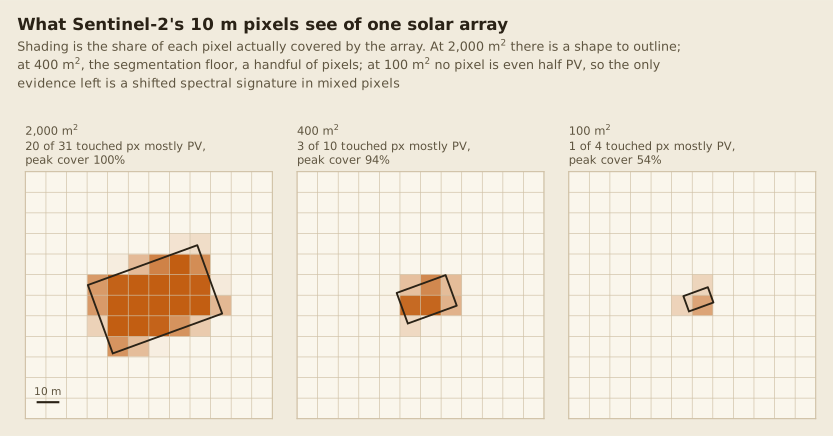
• Above roughly 400 m² an array has a shape, so detection works in the spatial domain: the fine-tuned TerraMind model labels each pixel and its outline becomes a candidate polygon. The detection model page walks through this on real installations, from a utility plant the model cannot miss to a 715 m² rooftop it usually does.
• Below the floor an array is a fraction of one mixed pixel, so detection moves to the spectral domain: a panel-covered roof is a few percent darker than the same roof without panels, deepest in red and near-infrared, with a slight blue tint and a relative SWIR excess. No outline exists, so the rooftop classifier scores whole buildings on that signature instead, and its skill is measured on exhaustively mapped calibration quadrats. How roofclf sees panels explains why silicon makes a roof darkest in the near infrared.

Neither domain proves an individual roof. The spatial detector tolerates false positives because a person reviews every lead; the spectral detector is never read per building at all, only summed into calibrated adoption rates. Both of those design choices follow from the physics in the figure above.

Where the spectral detector stops working

The physics above has a boundary, and France measured it. roofclf reaches 0.857 AUC in Pakistan and 0.710 in France, 0.821 against 0.627 once building size is controlled for. The interesting part is which explanation survives measurement, because the obvious candidates do not.

It is not the buildings. French roofs carrying PV are essentially the same size as Pakistani ones. What differs is what sits on them:

	Median PV-bearing roof	Median array on it	Array's share of its roof
Pakistan	195 m²	54 m²	0.309
France	202 m²	24 m²	0.119

A Pakistani array covers about a third of its roof; a French one about an eighth. That ratio, not the building, is what a mixed pixel responds to, and the feature ablation shows it directly:

	Pakistan	France
Footprint size only	0.744	0.673
Reflectance only	0.833	0.672
Size and reflectance together	0.857	0.710
What reflectance adds over size	+0.113	+0.037

In Pakistan reflectance alone reaches 0.833: the sensor genuinely sees panel. In France reflectance alone is 0.672, indistinguishable from footprint size alone at 0.673, so the French model is a building-size model with a spectral decoration on top. The dilution reading is supported by an external control: the same installations are recovered at 0.67 from sub-metre imagery with no size gradient, so the signal is present in the scene and averaged away by the pixel, rather than genuinely ambiguous.

The regime is set by policy, not by landscape. The France-Germany border is the natural experiment, since climate and building stock are continuous across it and feed-in tariff history is not.

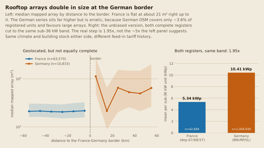
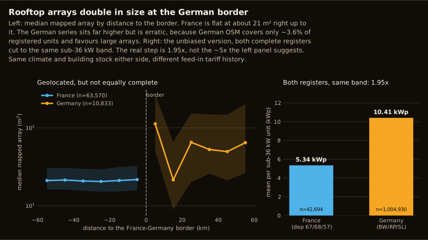
French installations do not grow as they approach Germany. They sit at 20.5 to 21.7 m² in every ten-kilometre band out to 60 km, and then the step happens at the line itself.

How big the step is depends entirely on which instrument you ask, which is why the figure carries two panels. The geolocated comparison suggests roughly 5x, but its German side is OSM at ~3.6% completeness and mappers trace large arrays first. Cutting both complete registers to the same sub-36 kW band gives the unbiased answer: 5.34 kWp per unit in Alsace and Moselle against 10.41 in Baden-Wuerttemberg, Rhineland-Palatinate and Saarland, a factor of 1.95 over 42,694 and 1,004,930 units. Real, large, and half what the imagery-based comparison implies.

That is the practical warning for any new country: the size regime, and therefore whether roofclf can work at all, is a property of national subsidy design rather than of geography, so it cannot be inferred from a neighbour.

Three plausible fixes have been measured, and two of them do nothing.

Fix	Effect on French AUC within size band
13x more training labels, from OpenPVMapper	-0.010
Authoritative footprints (French cadastre instead of VIDA)	+0.027
Retraining segmentation on 18,577 French chips	no change in recall (0.0118)

The footprint result is worth keeping even though it does not rescue the instrument: VIDA is imagery-derived and in these communes finds 44,314 buildings where the DGFiP cadastre finds 103,697, missing 58% of buildings and 30% of the PV-bearing ones. Better footprints are a real improvement to feature quality, and they close 14% of the gap to Pakistan. The remaining 86% is the sensor.

What this means for reading the atlas. The sub-400 m² half of the method is calibrated on installations that are small relative to the 400 m² segmentation floor but still large relative to a 100 m² pixel. Where that stops being true, the instrument stops working, and France has no roofclf half in its atlas for exactly this reason. The nearest thing to the French regime inside Pakistan is the sparse-density stratum, already the least well supported part of the coverage-ratio fit, and it should be read with this in mind.

Two products fall out of one model

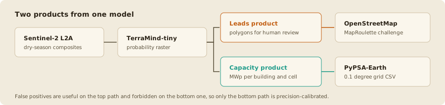
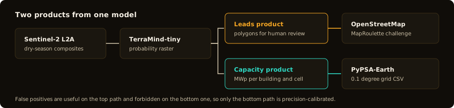
The split matters because the two products have opposite tolerances. On the leads path a false positive is cheap and a miss is expensive, so the model runs hot. On the capacity path there is no human in the loop at all, so every candidate is reweighted by a measured probability of being real before its area is counted. Same rasters, different accounting, documented in Calibration.

Reproducing the loop

Every step above is a CLI command that is resumable and safe to re-run. The full runbook, including how to start on a region with no pre-existing data, is in Setup New Country.

Architecture

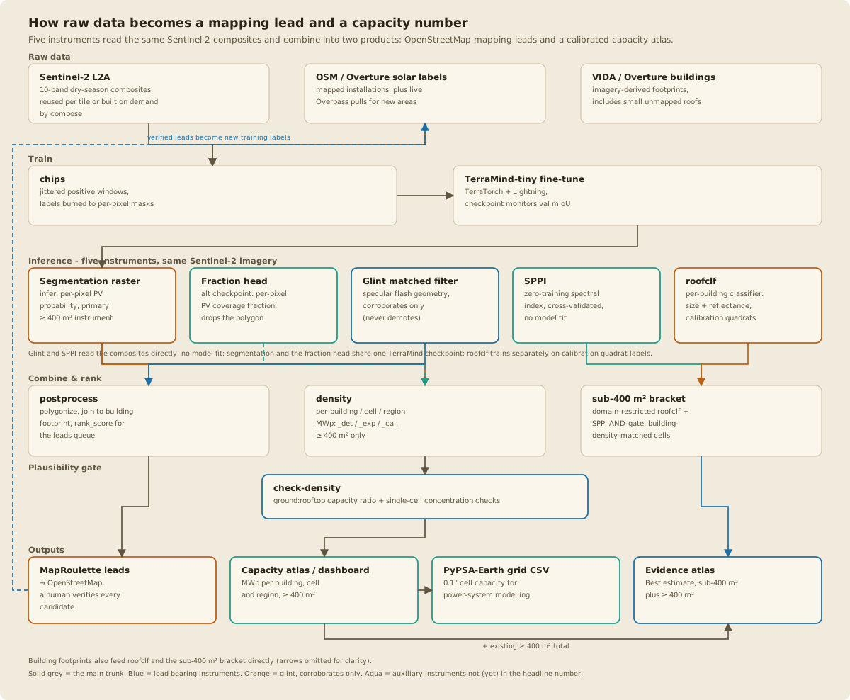
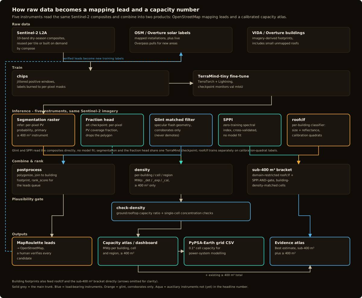
Workflow tells the human story: OpenStreetMap labels a model, the model proposes leads, mappers dispose of them, and verified installations become the next round of labels. This section is the technical complement: what actually reads what, stage by stage, from raw Sentinel-2 pixels to the two published products. Each box below is a real module or CLI stage; the Setup New Country runbook runs them in this order.

Raw data, once

Three inputs, each reused everywhere downstream rather than re-fetched per stage:

• Sentinel-2 L2A -- 10-band dry-season composites (local_source.py's CompositeIndex where a sibling project already downloaded a tile, otherwise compose.py builds one on demand from Planetary Computer STAC). Every instrument in the inference lane reads from this same set of rasters.
• OSM / Overture solar labels -- mapped installations from Overture's periodic snapshot, or a live Overpass pull for a region being freshly mapped (earthpv overpass-labels). This is both the training signal and, through the flywheel, the destination the pipeline's own output eventually feeds back into.
• VIDA / Overture buildings -- imagery-derived footprints (buildings.py), which matter because they include small, unmapped structures OpenStreetMap does not yet have. Buildings feed three downstream consumers directly: postprocess's building join, roofclf's per-building features, and the sub-400 m² bracket's domain restriction. The diagram omits those three arrows to stay legible; the dependency is real in all three places.

The main workflow and what's optional

chips cuts jittered training windows and burns label polygons into per-pixel masks; train fine-tunes terramind_v1_tiny through TerraTorch into a checkpoint that monitors validation mIoU. See Detection model for the model internals and the two invariants (chip jitter, Hann-tapered overlap-add) that keep inference from tiling into a grid of false positives.

From there, five instruments can read the same Sentinel-2 composites, but only two of them are the main workflow -- everything else is optional, kept as evidence, a secondary product, or a documented negative result:

Instrument	Part of the main workflow?	Needs the trained checkpoint?	What it outputs
Segmentation raster (infer)	Yes -- every mapping lead; all ground-mount capacity; rooftop ≥ 400 m² outside roofclf's calibrated cells	Yes, the primary one	per-pixel PV probability; the only instrument with a polygon and a defended ≥ 400 m² floor
roofclf	Yes -- every rooftop < 400 m², plus rooftop ≥ 400 m² inside its calibrated cells, where it replaces segmentation	No, a separate lightweight classifier	per-building "does this roof carry PV," trained on exhaustively mapped calibration quadrats
SPPI (spectral PV probability index)	Partially -- cross-checks roofclf as an internal floor for the evidence atlas	No, a fixed spectral formula	a zero-training index, cross-validated against the same ground truth as roofclf
Glint matched filter	Optional -- boosts the leads ranking only	No	specular-flash geometry consistent with one fixed panel plane; a physical corroboration, not a probability
Fraction head	Optional, not promoted (see below)	Yes, a separately trained checkpoint	per-pixel PV coverage fraction; drops the polygon, aims at sub-400 m² signal a segmentation threshold cannot see

Glint and SPPI need no model fit at all. roofclf is trained, but on a different, much smaller, hand-labelled corpus (the calibration quadrats), not on the segmentation checkpoint. This matters for how much to trust agreement between instruments: two signals that share no training data corroborating each other is real evidence; two heads of the same checkpoint agreeing is not.

Two optional instruments never got promoted past "evidence"

The fraction head and standalone SPPI are marked in the diagram as auxiliary: each carries real signal, but roofclf already does its job with a calibration measured on the quadrats. Neither is part of the main workflow, and the main workflow does not need them to be:

• The fraction head recovers far more sub-400 m² PV area than segmentation (0.520 of mapped area against 0.023 in Lahore DHA, 0.042 against 0.000 in Karachi coastal), but its predicted/true ratio spans 0.042 to 2.077 across quadrats, a quadrat-supervised retrain that looked consistent in sample did not hold on its holdout, and as a roofclf input it lowers AUC on small buildings. It is therefore not in the evidence atlas; it appears only in the directional growth map. The check-density failure first blamed on it happened without it too and has since been fixed.
• SPPI beats roofclf on nothing (median AUC 0.823 against 0.874 on the same nine-quadrat evaluation; roofclf reaches 0.879 on the full 27-quadrat set it is fitted on) and adds nothing as a roofclf feature, but an AND-gate (roofclf and SPPI agreeing) raises precision by 4 points at matched recall in the three quadrats where roofclf alone overestimates. That AND-gate is what the evidence atlas uses as an internal floor so the headline figure never reads below what a person has actually mapped plus that stricter population -- SPPI's one load-bearing role in the main workflow, short of being a standalone instrument in it.

Glint is the one instrument in the "boosts only" lane: it can raise rank_score, never lower it, because a missing glint on a real array (bad viewing geometry, wrong season) is common, while a glint on something that is not PV is rare. It is optional -- the leads queue and the evidence atlas both work without it -- but costs nothing to leave on. See Solar glint and Panel pose from glint.

Combine, rank, and gate

• postprocess polygonizes the segmentation raster, joins each candidate to a building footprint, and computes rank_score -- the ranking the leads queue is sorted by. Glint corroboration boosts this score; nothing here demotes a candidate to zero, because a false positive on this path costs a mapper seconds and a miss is invisible forever.
• density aggregates the same candidates into per-building, per-cell and per-region MWp using three metrics (*_det, *_exp, *_cal) described in Capacity density. This is segmentation's own ≥ 400 m² total, rooftop and ground-mount; below that floor the recall correction cannot rescue what was never detected, and ge400-roof-capacity below supersedes its rooftop component wherever roofclf has been calibrated.
• roof-classifier → roofclf-score-national → sub400-capacity fits roofclf on the calibration quadrats, scores every VIDA building nationally, then restricts to the 2,957 of 4,463 cells whose building density matches the quadrats and intersects roofclf with SPPI, explicitly refusing to rescale that figure to a national total. It covers roofclf's < 400 m² population, a separate module (sub400_capacity.py) not merged into density.py.
• ge400-roof-capacity applies the same domain restriction and coverage-ratio conversion to buildings roofclf flags at or above 400 m², and its output replaces density's own rooftop estimate for those buildings, inside those same cells only -- measured better there (0.896 AUC against segmentation's 0.73-0.78 on identical buildings). Outside the calibrated cells, and for every ground-mount candidate, density's own segmentation-based figure stays authoritative. Both functions feed the same evidence atlas. The rooftop classifier walks the whole path, from a hand-mapped square kilometre to the atlas numbers, with a flow chart.
• check-density (plausibility.py) is the only automated check between density and publishing: a ground-mount-to-rooftop capacity ratio per region and a single-cell concentration check, both tuned so the pre-fix 18.3 GWp Pakistan run (Gilgit-Baltistan 166 MWp of ground-mount against 0.8 MWp of rooftop) fails and the current run passes. It has no CI hook -- data/ is gitignored, so a human must run it.

The outputs: leads, the evidence atlas, and what else comes out

Everything converges on the main workflow's two outputs, plus optional extras built from the same underlying artifacts:

• MapRoulette leads → OpenStreetMap (main workflow). Every candidate, ranked, with a human verifying each one before it becomes a map edit. False positives are cheap here.
• The evidence atlas (main workflow, and this project's primary output). Reports Best estimate, this project's own highest defensible figure: hand-mapped OSM installations, plus segmentation's ground-mount detections, plus rooftop ≥ 400 m² from roofclf inside its calibrated cells and from segmentation elsewhere, plus roofclf-alone density below 400 m², plus a smaller roofclf-and-SPPI extension outside the calibrated cells -- OSM overlap removed rather than double-counted throughout, and floored per cell at what a person has actually mapped plus the stricter roofclf-and-SPPI agreement population. An earlier, looser tier, Ceiling (a flat-precision, uncalibrated upper bound), was removed on 2026-08-06: a later roofclf refit's lower deployment threshold roughly doubled it with no accompanying validation, so it had stopped being a meaningful bound.
• PyPSA-Earth grid CSV (a byproduct of the main workflow's density stage, no extra computation). No human in the loop, so every candidate is reweighted by a measured probability of being real (configs/calibration/) before its area counts. See Calibration.
• Optional extras, same artifacts, not required for the above: the plain segmentation- only capacity atlas (earthpv atlas with no --sub400-* flags, what a country with no mapped quadrats yet gets), the older Low/Central/High/All-PV bracket atlas, the rooftop potential/saturation atlas, and the retired config-driven national dashboard bundle (earthpv dashboard, kept working but no longer built by this site -- Results links directly to each standalone artifact page instead).

Where each stage is documented in depth

Stage	Main workflow?	Module	Read next
Labels, buildings	Yes	labels.py, overture.py, buildings.py	Scale to a new country
Chips, train, infer	Yes -- the segmentation checkpoint every polygon comes from	chips.py, train.py, infer.py	Detection model
postprocess, export	Yes -- every mapping lead, any size	postprocess.py, export.py	Segmentation & the building map
density, calibration	Yes -- segmentation's ≥ 400 m² total, rooftop and ground-mount	density.py, capacity_calibration.py	Capacity density, Calibration
roofclf, SPPI	Yes -- < 400 m² rooftop, plus ≥ 400 m² rooftop inside the calibrated cells	roofclf.py, sub400_capacity.py, roofclf_ge400_capacity.py	The rooftop classifier, Calibration quadrats
Plausibility gate	Yes	plausibility.py	this page's Combine, rank, and gate section
Atlas	Yes -- the evidence atlas, the primary output	atlas.py	Capacity map, Growth
Glint	Optional -- boosts leads ranking only	glint.py	Solar glint, Panel pose

Methods

The stages above have their own deep-dive reference pages, kept separate from this narrative overview because several of them (capacity density especially) are substantial technical documents in their own right:

Page	What it covers
Detection model	The TerraMind fine-tune, chip jitter and the tiling invariants that keep inference from gridding into false positives
Capacity density	The four capacity metrics, recall correction and credible intervals, the sub-400 m² bracket, and the plausibility gate
Solar glint	The physical glint-corroboration signal, with an image gallery
Calibration	How raw candidate area becomes a defended, probability-weighted capacity number
Calibration quadrats overview	Current status of every hand-mapped ground-truth quadrat
Quadrat protocol	How to map a new calibration quadrat to the standard the others were held to

Experiments

Most of what has been tried in this project did not ship, and the negative results are the map of where Sentinel-2's 10 m resolution limit actually sits. That record has its own page rather than a section here:

• Experiments -- the full register, with a verdict on each and the measurement behind it. Everything from the in-domain training chips that tripled recall to the three super-resolution variants that did nothing, plus links to every deep write-up.