Setting up a new country¶

Pakistan is the first pilot, not the product. Every input this pipeline needs is a global open dataset, and the model was trained in Germany before it was ever pointed at Punjab -- nothing about the setup below is Pakistan-specific. This page is also, incidentally, how every number on this site was produced: every stage is resumable and safe to re-run, so the same commands that bring up a new country also reproduce Pakistan's own results. Most real runs here are network-bound or GPU-bound for hours.

Requirements¶

An NVIDIA GPU for training and inference. The project targets a GTX 1060 (Pascal, sm_61), which is why PyTorch is pinned to cu126 wheels: CUDA 13 dropped Pascal support. Anything newer works and needs no change.
Disk. data/ is gitignored and expected on a fast local or external drive. Chips, composites, models and predictions run from multi-GB to multi-hundred-GB.
Nothing else. The already-configured AOIs reuse imagery a sibling project downloaded on the development machine, but that is a shortcut, not a requirement, and running on a new region covers the standalone path.

Install¶

pixi install              # data pipeline: DuckDB, geopandas, rasterio, odc-stac
pixi install -e ml        # adds PyTorch cu126 and TerraTorch, a multi-GB solve
pixi run -e ml gpu-check  # confirms torch.cuda.is_available() and the device name

Two environments share one solve group. default has no PyTorch and covers every data and network stage; ml adds torch and terratorch and is only needed for train, infer, evaluate and hard-negatives. On long runs, calling .pixi/envs/ml/bin/python -m earthpv.cli ... directly skips pixi's per-invocation overhead.

A third environment, docs, builds this site and is independent of both.

Smoke test first¶

A complete, minutes-long pass through every stage that touches the GPU. Do this on a fresh checkout before committing to a multi-hour run.

pixi run earthpv labels --aoi freiburg                    # tiny bbox, seconds
pixi run earthpv chips  --aoi freiburg --limit 50         # 50 chips, about a minute
pixi run -e ml earthpv train --config configs/terramind_pv.yaml --smoke
pixi run -e ml earthpv evaluate --aoi freiburg --checkpoint data/models/last.ckpt

--smoke runs 50 optimizer steps. That is enough to confirm the model loads, the GPU is used and a checkpoint is written, and nowhere near enough to detect anything. Do not read anything into the evaluate numbers here.

The full pipeline¶

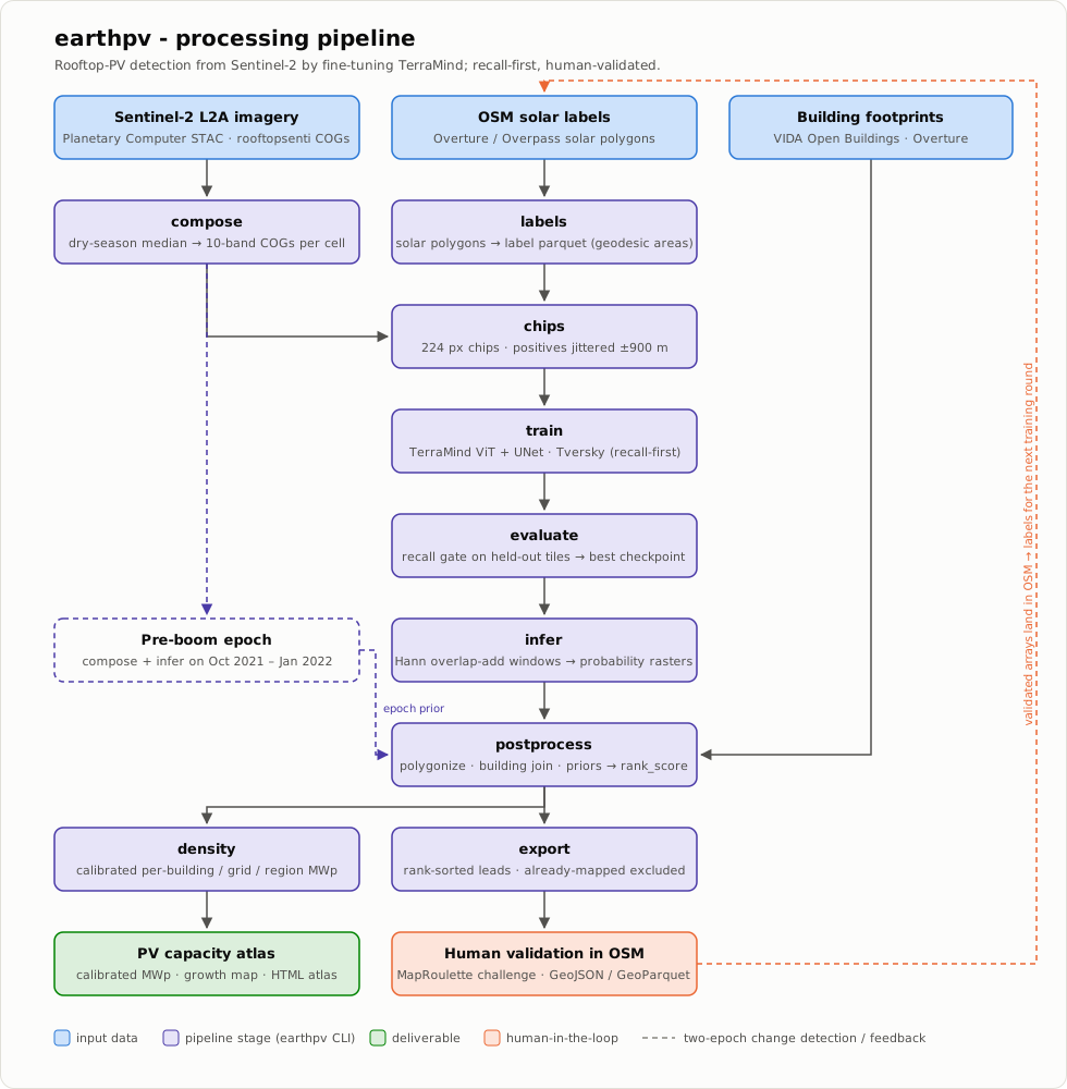
Ordered by dependency. Every stage after train needs a checkpoint path. Steps 1-15 are the project's default, main workflow -- segmentation for individual arrays ≥ 400 m² (steps 6-9), roofclf for every building below that floor plus its own ≥ 400 m² rooftop replacement (steps 10-14, including the essential random-cell manual validation at step 12), combined by step 15 into the evidence atlas, which is this project's primary output. Step 16 (Germany calibration and validation) and everything in the experiments register are optional extras, not alternative main paths.

1. Labels2. Chips3. Train4. Evaluate5. Compose6. Infer7. Postprocess8. Export9. Density10. Roof classifier11. Score roofclf nationally12. Manual validation (random cells)13. Sub-400 m² capacity14. ≥400 m² rooftop capacity (roofclf)15. Evidence atlas16. Germany calibration and validation (optional)

Building footprints and OpenStreetMap solar polygons for an area.

pixi run earthpv labels --aoi germany

# Freshly mapped region, bypassing Overture's snapshot lag, for example right
# after a mapping session:
pixi run earthpv overpass-labels --place "Lahore" --iso3 PAK

Country-scale Overpass fetches need per-province chunking or they time out.

Sentinel-2 composite windows with PV masks burned in: the training set.

pixi run earthpv chips --aoi germany                # full run, 3 to 4k chips
pixi run earthpv chips --aoi germany --limit 500    # capped, for iteration
pixi run earthpv chips --aoi germany --fraction     # continuous coverage-fraction target

pixi run -e ml earthpv train --config configs/terramind_pv.yaml

# Merge several areas into one training set first. The `:2` oversamples Pakistan's
# rows so Germany's larger chip count does not swamp the in-domain signal.
.pixi/envs/default/bin/python scripts/merge_chip_index.py germany pakistan:2

Pixel IoU and F1, plus per-installation recall bucketed by array size.

pixi run -e ml earthpv evaluate --aoi germany \
    --checkpoint data/models/<run>/<epoch>.ckpt

Build Sentinel-2 composites for areas with no local imagery. Skip for areas whose source_region already has them.

pixi run -e ml earthpv compose --aoi punjab --min-buildings 1000 --workers 6

# A second epoch on the same grid, here the pre-2022-boom baseline:
pixi run -e ml earthpv compose --aoi pakistan --index 1 \
    --window 2021-10-01:2022-01-24 --use-vida --workers 6

The pre-boom window deliberately ends 2022-01-24 to stay on one Sentinel-2 processing baseline: the 04.00 change in January 2022 shifts the digital-number convention by +1000 mid-window.

Tiled inference writing one probability GeoTIFF per cell.

pixi run -e ml earthpv infer --aoi punjab \
    --checkpoint data/models/<run>/<epoch>.ckpt

Threshold, polygonize, join to buildings, rank.

pixi run earthpv postprocess --aoi punjab --threshold 0.3

# Drop isolated candidates far from any building:
pixi run earthpv postprocess --aoi punjab --threshold 0.3 --max-building-dist 30

# Physics-based glint corroboration, calibrated and budgeted:
pixi run earthpv postprocess --aoi punjab --check-glint \
    --glint-top-n 300 --glint-skip-top 100

GeoParquet, GeoJSON and a MapRoulette challenge, ordered by rank_score.

pixi run earthpv export --aoi punjab

# New leads only, excluding anything within 100 m of mapped OpenStreetMap solar:
pixi run earthpv export --aoi punjab --exclude-mapped --min-distance-m 100

# Plus the pre-boom and vegetation vetoes, into new_leads_clean:
pixi run earthpv export --aoi punjab --exclude-mapped --min-distance-m 100 \
    --epoch-clean --veg-max-ndvi 0.35

Per-building PV area and capacity for the ≥ 400 m² segmentation half of the main workflow, plus grid and region aggregates. No GPU, no retraining, runs on artifacts already on disk.

pixi run earthpv calibrate-candidates --aoi pakistan
pixi run earthpv density --aoi pakistan --districts

# Gate the numbers before publishing them: exits non-zero if a province's
# ground-mount estimate dwarfs its rooftop one, or if one cell dominates a region.
pixi run earthpv check-density --aoi pakistan

# Optional precision upgrade for the bins below 1,000 m2, where glint is blind:
pixi run earthpv calibrate-sample --aoi pakistan     # fill `verdict` in JOSM or QGIS
pixi run earthpv calibrate-candidates --aoi pakistan --manual-reviews <reviewed file>

Changing --max-candidate-m2 or either --kwp-per-m2-* constant only reaches the per-building and *_roof columns on a --force re-run, which rebuilds every cell partial and takes about two hours for Pakistan. The candidate-population columns (*_total, *_roofcand, est_mwp_rc) are rederived on every run.

If your AOI has no mapped calibration quadrats yet, stop here and run step 15 without any --sub400-*/--ge400-roof-cells flag: that gives the ≥ 400 m²-only atlas, which is still this workflow's output for that country -- steps 10-14 need quadrats to exist first.

The < 400 m² half of the main workflow: a per-building "does this roof carry PV?" classifier, fit on the exhaustively mapped calibration quadrats (the only source where a no-PV building is a real negative -- see the quadrat protocol). No GPU. The rooftop classifier explains what steps 10 to 14 are doing and why, with a flow chart.

pixi run earthpv roof-classifier --aoi pakistan

Writes data/roofclf/: model_full.json (the pooled fit every later step reads), summary.json (leave-one-quadrat-out AUC and the precision-targeted deployment threshold), folds.csv and buildings.geoparquet. Reports skill per quadrat, never pooled -- see Capacity density for why a pooled number here would be misleading.

Add --parcel-label to count mapped PV in each building's 20 m yard as well as on its roof (the parcel label). It changes what every downstream coverage-ratio and area-recall correction measures, so use a separate --out-dir and rescore nationally against that model before running sub400-capacity. --table-path <buildings.geoparquet> refits from an existing table without rebuilding all 27 quadrats, which is the cheap way to compare feature sets.

Apply the fitted model to every VIDA building in the AOI. No GPU, but the long pole of the main workflow at country scale.

pixi run earthpv roofclf-score-national --aoi pakistan

Resumable per cell (--force to redo one that already exists) and safe to run detached -- see Operational notes below; at Pakistan's ~4,470 cells this takes 2 to 3 hours. Writes one parquet per cell (p_roofclf, sppi) to data/roofclf_national_with_sppi/<aoi>/prob/.

Essential, not optional -- run this after every national scoring pass, not just once. The calibration quadrats are curated and industrial-leaning; this is the un-curated counterpart, a fresh random sample of national cells reviewed by hand in JOSM. See Random-cell manual validation for the full protocol (selection, JOSM review steps, and where to record what you find) -- this is just the command:

pixi run roofclf-tiles -- --random-cells 20 --seed 1 --mapcss

No GPU. Writes complete, un-sampled GeoJSON tiles to results/<aoi>_roofclf_validation/, one region per drawn cell, in the exact format --all-quadrats already uses. A fresh --seed each run draws a new, independent batch -- the point is repetition over time, building up a precision estimate on a population the quadrats cannot represent by construction.

--random-cells draws from every scored cell nationally, not from the density-matched domain step 13/14 actually restrict capacity to -- a batch can land entirely outside it by chance (measured 2026-08-10: the first-ever batch did). Draw a domain-aware batch instead by passing an explicit --cell list computed from sub400_capacity.national_cell_domain; see Random-cell manual validation (its "first batch drew zero domain-matched cells" section) for the exact recipe and why both an in-domain and an out-of-domain batch matter.

Restrict the national scoring to cells whose building density matches the calibration quadrats, dedupe against existing segmentation candidates and mapped OSM solar, and convert to capacity at the LOQO-measured precision. No GPU.

pixi run earthpv sub400-capacity --aoi pakistan \
    --osm-solar data/labels/pakistan_overpass_solar.parquet

Writes three building-level parquets to data/roofclf_national_with_sppi/<aoi>/ density/: sub400_central_incremental_buildings.parquet (roofclf alone, the evidence atlas's Best-estimate small-PV component), sub400_low_incremental_ buildings.parquet (roofclf AND SPPI agreeing, used as an internal floor on Best estimate), and (added 2026-08-11) sub400_outdomain_and_gate_incremental_buildings.parquet (roofclf AND SPPI agreeing OUTSIDE the density-matched domain -- an extrapolation, no longer fed into the published atlas as of 2026-08-15, see step 15). The first two describe only the density-matched cells and must not be rescaled by their share of the country; the third describes the rest of the country and is even less certain, since no calibration quadrat sits in that density range at all. See sub400_capacity.py's module docstring and Capacity density for exactly what each does and does not claim.

roofclf replaces segmentation's own rooftop estimate for ≥ 400 m² buildings inside the SAME density-matched domain step 13 uses (roofclf measured AUC 0.896 vs segmentation's 0.73-0.78 on identical buildings -- segmentation is a weak instrument for small PV including small PV on large buildings). Ground-mount is untouched -- roofclf has no footprint to score there. No GPU.

pixi run earthpv ge400-roof-capacity --aoi pakistan \
    --osm-solar data/labels/pakistan_overpass_solar.parquet

Writes ge400_roof_incremental_buildings.parquet to data/roofclf_national_with_sppi/<aoi>/density/, feeding --ge400-roof-cells in the next step. Also not a national figure -- same domain-restriction caveat as step 13.

Combine both halves into the main workflow's primary output: Best estimate, de-duplicated against hand-mapped OSM.

pixi run earthpv atlas --aoi pakistan \
    --sub400-central-cells   data/roofclf_national_with_sppi/pakistan/density/sub400_central_incremental_buildings.parquet \
    --sub400-low-cells       data/roofclf_national_with_sppi/pakistan/density/sub400_low_incremental_buildings.parquet \
    --ge400-roof-cells       data/roofclf_national_with_sppi/pakistan/density/ge400_roof_incremental_buildings.parquet \
    --osm-solar data/labels/pakistan_overpass_solar.parquet \
    --pose-summary-csv data/glint/country2000_summary.csv \
    --pose-history-note "(a 4x-larger, chunked-tile-batch re-run of the original 500-target study)" \
    --pose-data-note "(2000-target stratified country study, chunked tile-batch pull)" \
    --imagery-date-range "Oct 2025 - Jun 2026" \
    --downloads-manifest configs/pakistan_atlas_downloads.json \
    --data-release-url https://github.com/open-energy-transition/earthpv/releases/download/pakistan-atlas-data-2026-08-14 \
    --out docs/assets/interactive/pakistan_evidence_atlas.html

--downloads-manifest/--data-release-url write a collapsed "Download the underlying data" section at the very bottom of the page -- capacity parquets, calibration boundaries, the pose survey, raw detections, and the model checkpoint, hosted as assets on a dated GitHub Release rather than in data/ itself (which is gitignored). --downloads-manifest is a JSON file of {file, label, note, size_bytes} dicts (see configs/pakistan_atlas_downloads.json for the Pakistan manifest); --data-release-url is the release's asset base URL, joined with each entry's file to build its link. Both are a frozen, point-in-time snapshot -- the manifest is not regenerated automatically when the pipeline reruns, so a fresh data drop needs a new GitHub Release plus an updated manifest and --data-release-url. Omitting either flag omits the section entirely. The section also always shows a short Overpass query for the current, live state of OSM-mapped PV, since the raw detections in the release will go stale as mappers keep editing.

--imagery-date-range is a free-text label, not a derived value -- composites for this AOI mix cells earthpv compose fetched directly with cells reused from a source_region cache built by a different project on its own schedule, so there is nowhere in the pipeline that already knows the combined answer; it has to be supplied by whoever last checked. The page always stamps its own build date regardless of whether this is given.

Two optional sections. A "Capacity per size bin, rooftop vs ground-mount" chart (the same re-binning atlas-by-size publishes as its own page, computed from this run's own inputs so the two numbers can't drift by construction) is embedded natively whenever --ge400-roof-cells is given -- no separate flag needed. --pose-summary-csv additionally embeds the panel-pose survey (docs/results/pv-pose.md, earthpv.pose.compute_pose_survey_data) natively too, scoped under its own .pose-native CSS namespace so nothing leaks onto the rest of the page. --pose-history-note/--pose-data-note are optional strings passed straight through. Omitting --pose-summary-csv writes the page with no pose section at all.

--sub400-outdomain-cells is optional and the published atlas does not pass it -- it would add roofclf-AND-SPPI agreement outside the density-matched domain to Best as a strict, clearly-marked extrapolation, but that component is not measured where it would be applied and the JOSM pass meant to check it is blocked by stale reference imagery. See Capacity map for why. Both sub400-* and this flag's input come from step 13's earthpv sub400-capacity, which writes all three building-level parquets in one run.

--ge400-roof-cells is easy to omit by accident and changes the headline number by double digits of percent (measured 2026-08-10: omitting it dropped Best estimate 14.6%) -- it is a separate step (14) from the rest of the atlas's inputs, unlike --sub400-*, which both come from step 13. --out matters too: without it, the atlas writes to data/predictions/<aoi>/density/<aoi>_pv_evidence_atlas.html, not this project's actual published location (docs/assets/interactive/pakistan_evidence_atlas.html, what the docs site and README screenshot read).

Best estimate combines hand-mapped OSM installations with recall-corrected ≥ 400 m² detections (roofclf's own estimate inside the density-matched domain from step 14, segmentation's recall-corrected estimate everywhere else) plus roofclf-alone density, with the OSM/detection overlap removed rather than double-counted, and floored per cell at hand-mapped OSM plus the stricter roofclf-and-SPPI agreement population. Without a mapped quadrat yet (step 10's prerequisite), omit --sub400-*/--ge400-roof-cells entirely for the ≥ 400 m² segmentation-only atlas -- still this workflow's output, just missing its sub-400 m² half until quadrats exist.

Optional, Germany only, and not part of the main workflow above. Germany is the one place with a legally complete register, so it is where the method's assumptions can be checked against ground truth rather than against another estimate.

pixi run earthpv mastr        # once: download and aggregate MaStR (multi-GB, hours)
pixi run earthpv calibrate --aoi germany       # calibrate a prob raster per Gemeinde
pixi run earthpv pv-yield --aoi germany        # pvlib GWh/yr cross-check

# Validate the methodology itself: how much capacity sits below the detection floor,
# how transferable that share is, and whether OSM can serve as a reference at all.
pixi run earthpv validate-mastr --aoi germany \
  --solar-path <a national OSM solar pull for Germany>

validate-mastr's register-internal checks need no imagery and run in under a minute. Its end-to-end per-municipality comparison needs a German density run, which is currently blocked on composites and a small-roof building layer; it reports its own coverage and refuses to call a partial-coverage result national. See Validation against MaStR.

Areas and their parameters live in configs/aoi.yaml; model and training configs in configs/*.yaml.

Running on a new region¶

The configured areas reuse locally cached imagery, which is a shortcut specific to the development machine. A region with no local data at all needs nothing pre-downloaded:

labels or overpass-labels fetch OpenStreetMap solar polygons directly, from Overture or live Overpass, instead of reading a cached parquet.
chips and compose fetch Sentinel-2 from Planetary Computer STAC. Same code path, just slower.
The building join fetches VIDA Open Buildings for the area's country on first use and caches it. Works for any ISO3 code.
Detection reuses the existing checkpoint unchanged. No region-specific retraining is needed for a first candidate set.

Three commands cover setup:

pixi run python scripts/new_region.py check --bbox <bbox> --iso3 <ISO3>   # preflight
pixi run python scripts/new_region.py add   --aoi <name> --bbox <bbox> --iso3 <ISO3>
pixi run python scripts/new_region.py plan  --aoi <name>                  # runbook

Scale to a new country below is the full guide: what to expect by starting condition and what differs from Pakistan.

Scale to a new country¶

This section is the path from "we would like a solar map of X" to a published capacity atlas for X. The programme's stated next targets are Mexico, Japan, Korea, Indonesia, India, Brazil, South Africa and Nigeria, and Gujarat in India is already registered as a worked template. None of them require anything Pakistan required.

What makes it portable¶

Input	Source	Coverage
Imagery	Copernicus Sentinel-2 L2A, via Planetary Computer or Earth Search	global, every five days, free
Labels	OpenStreetMap, via live Overpass or an Overture snapshot	global, wherever mappers have been
Building footprints	VIDA Open Buildings (Google and Microsoft)	global, imagery-derived, includes unmapped structures
Admin boundaries	geoBoundaries, CC-BY	global, ADM1 and ADM2
Model	TerraMind-tiny, fine-tuned, checkpoint in the repository	reusable as-is for a first pass

The one thing that is genuinely local is the human mapping community, and that is why the first step below is not a command.

Before you start: find the mappers¶

Detection produces leads. Leads only become data when somebody who knows the ground opens them in the OpenStreetMap editor and decides. In Pakistan that was four interns at the Lahore University of Management Sciences, and the difference they made is measurable: large-array recall in Punjab went from 0.18 to 0.55 purely on training data their verification produced.

A run with no mapping community attached gives you a candidate file nobody will validate, a recall number nobody can check, and a capacity estimate resting on a single global calibration. Line up a local OpenStreetMap community, a university group, or an NGO first. Community describes what that collaboration looks like.

Step 0: preflight¶

scripts/new_region.py check probes all four data sources before you commit any network time. It is read-only and takes a couple of minutes.

pixi run python scripts/new_region.py check \
    --bbox 98.5,7.8,101.0,10.2 --iso3 THA --name "Surat Thani"

[  ok  ] OpenStreetMap solar labels  412 features {'generator': 301, 'plant': 111}
[  ok  ] VIDA Open Buildings  available remotely, 6.9 GB
[  ok  ] geoBoundaries ADM1  Thailand
[  ok  ] geoBoundaries ADM2  Thailand
[  ok  ] Sentinel-2 imagery  336 scenes under 40% cloud across 16 MGRS tiles, median cloud 19%
[  ok  ] Grid size  600 cells of 0.1 degree over 72,943 km2

What the four answers actually tell you:

OpenStreetMap solar count. Zero is not a blocker for detection, but it means you have nothing to train on and nothing to measure recall against, so the capacity number will carry the global calibration's uncertainty rather than a local one. Under about 50 features, plan on mapping a quadrat early. Country-scale bboxes usually time out on Overpass; pass --skip-osm and query province by province instead.

VIDA availability. If the ISO3 code has no parquet, cell selection and the building prior both fall back to Overture, which undercounts small and informal structures by two to three orders of magnitude in exactly the places rooftop solar is growing fastest. Check the code before concluding the country is missing.

Imagery. The composite is a median of the least-cloudy scenes in a window, so a wet window gives a poor base. The default window tested is the northern dry season; adjust --window for the southern hemisphere or a monsoon climate. If the check reports no scenes under 40 percent cloud, pick a different window before anything else.

Grid size. A ceiling, not an estimate. Only building-populated cells get composited: in Pakistan that was about 4,470 of roughly 62,000, and at one to two minutes per cell that is the difference between a weekend and a month.

Step 1: register the area¶

pixi run python scripts/new_region.py add \
    --aoi surat_thani --bbox 98.5,7.8,101.0,10.2 --iso3 THA \
    --division "Surat Thani" --subtype region

That appends a block to configs/aoi.yaml, refuses to clobber an existing area, and re-parses the file so a malformed insert fails immediately rather than three stages later:

  # Added by scripts/new_region.py. No source_region key, so chips and compose fetch
  # from Planetary Computer STAC rather than a local composite cache.
  surat_thani:
    bbox: [98.5, 7.8, 101.0, 10.2]
    division: { name: Surat Thani, country: TH, subtype: region, iso3: THA }

The absence of a source_region key is what routes everything through the open fetchers. Areas that have one read a locally cached composite set instead, which is a shortcut specific to the development machine and not something a new region needs.

Always set iso3

VIDA and geoBoundaries are both keyed on ISO3. The ISO2-to-ISO3 fallback in buildings.py only covers the countries that predate this script, so a new area without an explicit iso3 will fail at the density stage rather than at setup. new_region.py add writes it for you.

Step 2: get the runbook¶

pixi run python scripts/new_region.py plan --aoi surat_thani

This prints the ordered command sequence with the area's name, bbox and ISO3 already substituted, including the systemd-run invocation for the long compose job. The rest of this section explains the reasoning behind those commands.

Step 3: first pass, no retraining¶

A first candidate set needs no local training data at all. The existing Germany-plus-Pakistan checkpoint runs unchanged.

# labels from live OpenStreetMap
pixi run earthpv overpass-labels --bbox 98.5,7.8,101.0,10.2 --iso3 THA --name surat_thani

# imagery, building-populated cells only, hours and network-bound
systemd-run --user --collect --unit=earthpv-compose-surat-thani \
  -p WorkingDirectory="$PWD" bash scripts/compose_loop.sh surat_thani 0 1000

# detect, rank, export
pixi run -e ml earthpv infer --aoi surat_thani \
    --checkpoint data/models/v2_combined/terramind-pv-epoch=39.ckpt
pixi run earthpv postprocess --aoi surat_thani --threshold 0.3 --max-building-dist 30
pixi run earthpv export --aoi surat_thani --exclude-mapped --min-distance-m 100

compose_loop.sh takes the area name, an optional target cell count (0 means run until compose finishes or stalls, which is what you want when the count is unknown) and the cell-selection threshold. It restarts compose every 30 minutes so a fresh Planetary Computer signing token replaces one about to expire mid-run.

Expect the first pass to be worse than Pakistan's. That is the domain gap, and it is the thing the next two steps close.

Step 4: map, and measure¶

This is the step that is easy to skip and expensive to skip.

Send the leads out. export writes a MapRoulette challenge sorted by rank. Mappers verify against the high-resolution layers and map what is real, which both improves OpenStreetMap and produces your training positives.

Map one quadrat exhaustively. Pick a 1 km² box in a built-up area and map every installation inside it, following the quadrat protocol. This is the only instrument that measures what the model misses. Leads tell you about candidates the model found; they cannot tell you about the installations it never proposed. The Lahore box is the reason the Pakistani recall estimate is now suspected of being optimistic, and it took one afternoon.

Review a calibration sample. earthpv calibrate-sample --aoi <area> emits a stratified sample of unmapped candidates for human verdicts. Twenty verdicts per size bin replace a wide extrapolated interval with a measured one.

Step 5: retrain in domain¶

Once mapping has produced local positives, the flywheel turns.

pixi run earthpv chips --aoi surat_thani
.pixi/envs/default/bin/python scripts/merge_chip_index.py germany surat_thani:2
pixi run -e ml earthpv train --config configs/terramind_pv.yaml
pixi run -e ml earthpv evaluate --aoi surat_thani --checkpoint <new checkpoint>

The :2 oversamples the new area so Germany's much larger chip count does not swamp the in-domain signal. Set val_tiles in configs/aoi.yaml to a geographically separate cluster before trusting any recall number: a validation split that overlaps the training cluster leaks through chip jitter and window overlap, and an empty val_tiles silently falls back to a random 20 percent split.

Step 6: capacity -- the main workflow's output¶

This is where the main workflow (steps 9-13 above) actually lands for a new country: segmentation's ≥ 400 m² total, plus roofclf's < 400 m² total once at least one quadrat exists, combined into the evidence atlas.

pixi run earthpv calibrate-candidates --aoi surat_thani
pixi run earthpv density --aoi surat_thani --districts
pixi run earthpv atlas --aoi surat_thani     # >= 400 m2 segmentation-only, for now

Without local calibration evidence the table marks itself status: interim-mapped-only and the capacity number is an honest lower bound. That is a legitimate thing to publish as long as you say so. See Calibration.

Once step 4's quadrat is mapped, extend to the full evidence atlas -- roofclf is what actually uses it:

pixi run earthpv roof-classifier --aoi surat_thani
pixi run earthpv roofclf-score-national --aoi surat_thani     # long: hours at country scale
pixi run earthpv sub400-capacity --aoi surat_thani \
    --osm-solar <national OSM/Overpass solar pull>
pixi run earthpv atlas --aoi surat_thani \
    --sub400-central-cells data/roofclf_national_with_sppi/surat_thani/density/sub400_central_incremental_buildings.parquet \
    --sub400-low-cells     data/roofclf_national_with_sppi/surat_thani/density/sub400_low_incremental_buildings.parquet \
    --osm-solar <national OSM/Overpass solar pull>

One quadrat is enough to fit roofclf and get a number, but leave-one-quadrat-out skill (what roof-classifier's summary.json reports) needs several, ideally spanning the region's different built-up densities the way Pakistan's do -- a single quadrat's number is not yet a measured skill estimate, just a fit. Quadrats and manual review are what turn the whole thing from a lower bound into an estimate with an interval. See Capacity density and Calibration.

Step 7: publish it on this site¶

Optional, and only relevant if the new country's results are meant to join this shared site rather than stay in your own deployment. Each new country's results are a short, hand-written page under docs/results/: a lede, an embedded interactive HTML page under docs/assets/interactive/ (INTERACTIVE in scripts/build_docs_figures.py is what copies it there -- add a (results/....html, docs-facing name) pair and run pixi run docs-figures), and a caveats section. docs/results/capacity.md and docs/results/growth.md are the templates to copy. Add the new page under mkdocs.yml's PV Atlas nav entry once it exists. There is deliberately no config schema or generator for this: a country's results are whatever pages it actually has, added by hand, not templated -- the one time this project tried a config-driven, auto-combined dashboard (earthpv dashboard, src/earthpv/dashboard.py), keeping it in sync turned out to cost more than the plain pages it replaced.

What to expect, by starting condition¶

Your region has	First pass gives you	What to do first
Dense OpenStreetMap solar already	Good recall, immediately useful leads	Retrain in domain; you have positives now
Some solar mapped, patchy	Moderate recall, many real new leads	Send leads out, map one quadrat
Almost nothing mapped	Low recall, unknown precision	Map a quadrat before anything else. Detection numbers are uninterpretable without one
A national PV register	The Germany situation	Calibrate against it, as `earthpv mastr` and `earthpv calibrate` do

Things that will differ from Pakistan¶

Climate and the composite window. A dry-season median is the right base in an arid climate. In a wet tropical or high-latitude region the least-cloudy twelve scenes may still be poor, and snow at high latitudes changes the background entirely. Test with new_region.py check --window before composing.

Roof type. Pakistan's dominant urban roof is flat concrete, which is why the roof-axis orientation prior failed there and why fitted panel tilts are bimodal. A region of pitched tile roofs behaves differently, and some priors that failed in Pakistan may work.

Glint geometry is latitude-dependent. Sentinel-2's overpass is at a fixed local time, so the range of panel orientations that can ever glint into the sensor is a function of latitude. The Pakistani pose survey could not observe anything west of due south. A different latitude has a different blind sector, and the southern hemisphere flips it.

Installation size distribution. The 400 m² floor bites hardest where residential PV dominates. In a region of large commercial rooftops, per-object detection covers far more of the capacity; in a region of 30 m² household systems, almost everything falls to the density stage.

Building data quality. VIDA is imagery-derived and its completeness varies. Where it is thin, the building prior weakens and --max-building-dist filtering gets riskier.

Reusing the model itself¶

The checkpoint under data/models/ is Germany plus Pakistan. For a region resembling either, use it directly. For one that resembles neither, the ordering that worked here was: train on the region with the best label quality available (Germany), infer on the target, have people verify, retrain with the verified target-region chips oversampled. That sequence, not a bigger backbone, is what moved the numbers.

Rebuilding this site¶

pixi run docs-figures          # charts, diagrams, logo variants, embedded pages
pixi run docs-screenshots      # re-capture the interactive pages as PNGs (needs firefox)
pixi run -e docs docs-serve    # live preview at http://127.0.0.1:8000
pixi run -e docs docs-build    # strict build into site/

scripts/build_docs_figures.py reads its numbers from files on disk wherever a file exists, so after a new pipeline pass the figures update themselves. Pushing to main publishes the site through GitHub Pages via .github/workflows/docs.yml.

scripts/screenshot_pages.py is separate because it needs a browser, which CI does not install. The README cannot embed an iframe, so its hero images are screenshots of the same interactive pages this site serves; re-run it after regenerating an atlas or pose page. If Firefox is installed as a snap it can only read a non-hidden directory under $HOME, so the script stages pages in ~/earthpv-screenshots/ before rendering.

Operational notes¶

These are the things that cost time on this project.

Long jobs die silently on logout

nohup setsid is not enough. systemd-logind kills a session's whole cgroup when the session ends unless lingering is enabled. Before launching anything multi-hour:

loginctl show-user "$USER" | grep Linger
loginctl enable-linger "$USER"     # once, no sudo needed for your own account

Run each long job as its own transient unit so one job's out-of-memory kill does not take the others with it:

systemd-run --user --collect --unit=earthpv-compose \
  -p WorkingDirectory=/path/to/earthpv bash scripts/compose_loop.sh

Planetary Computer has frequent multi-hour outages, either Azure Front Door 504s or requests that hang with no error at all. Every network-bound stage is resumable by design, with temp-then-rename writes and per-cell or per-target skip-if-exists. The practical pattern is to launch detached, poll a log for a completion marker or a stall of 20 to 30 minutes with no new output, and relaunch the same command if stalled. scripts/compose_loop.sh automates exactly that cycle, and also restarts every 30 minutes so a fresh signing token replaces one about to expire mid-run.

The progress bar does not flush to a redirected log. Watch checkpoint files or cell counts to gauge progress, not the log tail.

row.mask and row.image on a pandas row resolve to Series.mask, the method, not your column. Use bracket access, row["mask"]. This has caused real bugs here more than once.

Areas are geodesic (labels.geodesic_area_m2). Never call .area on latitude and longitude geometries; it silently returns square degrees.

Geographic validation splits must match real coverage. val_tiles in configs/aoi.yaml has to name MGRS tiles or composed cells the area actually produced, or the validation set is silently empty and the datamodule falls back to a random 20 percent split. Check that evaluate's reported installation count per bucket is not suspiciously small before trusting a recall number.

Changing MIN_PV_AREA requires rebuilding chips and retraining. It is baked into the burned masks, not a runtime parameter.

Orchestration scripts¶

Script	What it does
`screenshot_pages.py`	Render the interactive HTML pages to PNG with headless Firefox, for the README.
`new_region.py`	Preflight the four open data sources for a new area, register it in `configs/aoi.yaml`, print its runbook. See Scale to a new country.
`compose_loop.sh`	Auto-restarts `compose` every 30 minutes for a fresh token; exits on target reached, clean completion, or three no-progress cycles. Takes `[AOI] [TARGET_CELLS] [MIN_BUILDINGS]`.
`rebuild_training.sh`	Rebuilds an area's chips after its compose finishes, then remerges the combined training index.
`infer_after_compose.sh`	Waits for compose, then chains infer into postprocess into export.
`run_preboom_pipeline.sh`	The full two-epoch pipeline behind marker-file resumability.
`run_sr_experiments.sh`	The three super-resolution feasibility tests in sequence.
`download_vida_ind.sh`	Bulk VIDA India buildings download with retry on reset.
`build_docs_figures.py`	Every figure and embedded page on this site.

There is no test suite and no wired lint task. Ruff is configured at line length 100 and run manually. The practical "does it work" check is the smoke test above.