From raster to candidates: segmentation meets the building map

Detection model covers the model itself: what TerraMind is fine-tuned on, what it recovers, and the tiling invariants. This page covers everything that happens after the probability raster is written: how pixels become candidate polygons, how the building dataset classifies each one, and how that classification decides both a candidate's place in the mapping queue and the constant that converts its area to capacity. All of it lives in postprocess.py, entered by earthpv postprocess, and none of it needs a GPU.

The building dataset is not a garnish here. It is consulted at three separate points in the pipeline, and each consumer would be measurably wrong without it:

Consumer	What buildings decide there
This page: the candidate join	each candidate's placement, its ranking prior, and which kWp/m2 constant prices it
The rooftop classifier	the unit of prediction itself: roofclf scores one probability per footprint
Capacity density	per-building capacity attribution, capped at each building's own roof area

Step 1: from probability to polygons

polygonize_chips thresholds every per-cell raster at 0.3 and merges each connected group of surviving pixels into one polygon, carrying the group's peak probability as confidence. Areas are geodesic (labels.geodesic_area_m2), never planar degrees. Then two guards run before anything else sees the candidates:

• Polygons under 50 m² are dropped: at 10 m resolution that is a half-pixel sliver, below anything the model was meaningfully trained to resolve.
• Polygons over 100,000 m² are flagged oversize and later excluded from capacity. Merging every touching pixel has no upper bound, so one connected sheet of false positives can masquerade as a multi-km² "installation". A candidate whose geometry came from OpenStreetMap (next step) is exempt, because a human drew it.

The worked example on the detection page shows this operation on real installations, including the amber threshold contour.

Step 2: mapped geometry wins

Before the building join, replace_with_osm_geometry swaps a candidate's coarse polygonized blob for the real OpenStreetMap footprint where a mapped installation sits within 30 m. Only the closest OSM match per feature is used, so one mapped plant cannot be inherited by several nearby candidates, and the reference polygons are dissolved first so a power=plant perimeter with nested power=generator ways does not double-count one real installation. This runs early on purpose: the placement classification and the ranking below should both see the corrected geometry, not the blob.

Step 3: the building dataset

Footprints come from VIDA Open Buildings, a merge of Google Open Buildings and Microsoft Building Footprints. The property that matters is that it is imagery-derived: it contains the small, unmapped structures that OpenStreetMap in Pakistan largely does not, which is exactly the population a rooftop question needs. Pakistan's file is 76.6 million footprints; the join reads it windowed per area (the Parquet's own bounding-box index prunes to the candidates' extent) rather than loading the whole country. Where no VIDA layer exists for a country, the Overture ≥ 500 m² set is the fallback, at the cost of the metric distance signals below.

Step 4: the placement rule

Each candidate is joined to the footprints in its local UTM zone and classified by two numbers, its footprint overlap and its distance to the nearest footprint:

placement	Rule	Typical reality
rooftop	at least 30% of the candidate sits on a footprint	an array on an industrial or large residential roof
ground_adjacent	within 30 m of a footprint	a yard or compound array beside its building
no_building	neither	a ground-mount plant, or a false positive on bare ground

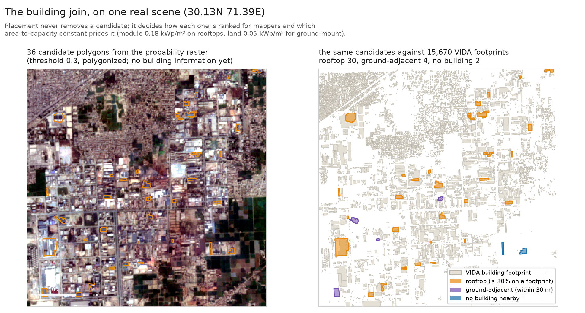
Nothing is removed at this step. The two no_building candidates in the figure stay in the export: one may be a real ground-mount plant and the other bare-ground glare, and on the leads path that distinction is a few seconds' work for a mapper, not the pipeline's call. (An optional --max-building-dist filter exists for exports where isolated detections are known to be noise; it is off by default and only applies where a real metric distance was resolved.)

Step 5: what placement is for

The classification earns its place twice, once on each product path.

On the capacity path it selects the conversion constant, and this is load-bearing. Rooftop detections convert at 0.18 kWp/m² of module area. Ground detections (ground_adjacent plus no_building) convert at 0.05 kWp/m² of site area, because ground-mount training labels are OSM power=plant perimeters: most of a plant's perimeter is spacing, roads and margins, not module. Applying the module constant to site area overstates ground-mount capacity by 2 to 3 times, and both constants are calibrated against real plants rather than assumed -- see Capacity density. The candidate-precision calibration is split by placement for the same reason: bright bare ground and industrial roofs are different false-positive populations, and pooling them lets one borrow the other's corroboration rate.

On the leads path it sets a prior, and the prior only reorders. A candidate's rank_score is its model confidence times (0.5 + 0.5 x prior), where the prior rewards sitting on a footprint (full weight once half the candidate is on a roof) or sitting just off one (decaying over tens of metres), and never falls below 0.15:

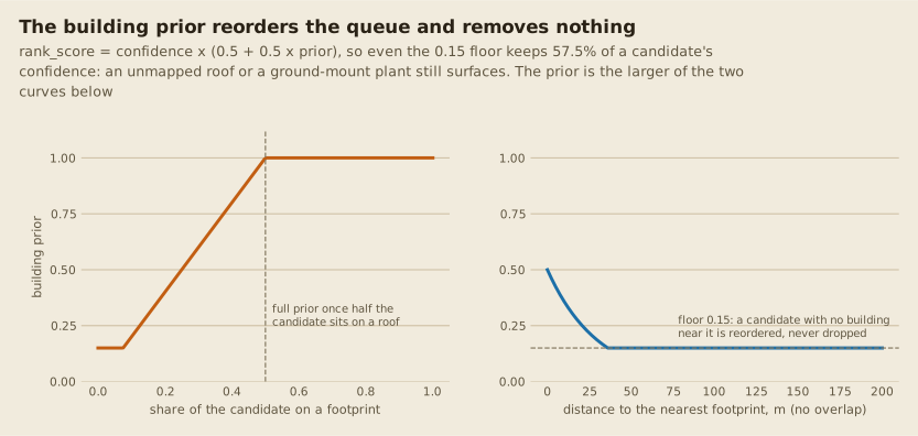
The floor is the recall-first contract in one number: even a candidate in open desert keeps 57.5% of its confidence, because an unmapped roof missing from VIDA and a ground-mount farm are both real targets. The same multiply-never-drop contract is shared by the two optional priors that can stack on top: the glint corroboration boost (up only) and the pre-boom epoch prior (down-weights candidates already bright in 2021 imagery, which are persistent false positives rather than new PV).

Step 6: two products, one candidate table

earthpv export sorts by rank_score and writes GeoParquet, GeoJSON and a MapRoulette challenge: the leads product, everything included, humans downstream. The same candidates, reweighted by the measured calibration instead of rank_score, feed earthpv density: the capacity product, nobody downstream, which is why it must not inherit the leads path's tolerance for false positives.

One property of the capacity path is worth knowing when reading its outputs: per-building capacity credits each building only with the candidate area that geometrically intersects its footprint, capped at the building's own roof area, while region totals count each rooftop candidate's full polygon once. Whitespace inside a rooftop-classified polygon therefore appears in region totals and not in building sums (a measured ~46% gap nationally), so any per-building disaggregation is a conservative, roof-anchored floor -- the full derivation is in Capacity density.

Read next

Topic	Page
The model that writes the probability raster	Detection model
How candidate area becomes defended capacity	Calibration, Capacity density
The per-building spectral instrument below 400 m2	The rooftop classifier
The glint boost this ranking can consume	Solar glint