The rooftop classifier (roofclf)

Shipped, and half the main workflow

roofclf is the instrument that covers everything below the segmentation model's 400 m² detection floor, and (inside its calibrated domain) it now also replaces segmentation's own rooftop estimate above that floor. Numbers on this page come from the 30-quadrat fit in data/roofclf/summary.json and the capacity run behind the published evidence atlas.

What it is, in one paragraph

roofclf is a per-building classifier that answers a single question: does this roof carry solar PV? It takes one building footprint, reads the Sentinel-2 pixels that fall inside it, and returns a probability. It never draws a panel outline, never says how many modules there are, and never looks at anything but that footprint and its own neighbourhood. It is a regularised logistic regression, about 17 numbers wide, trained on roughly a hundred thousand hand-checked buildings. It is deliberately the smallest model in this project.

Why the question changes at 400 m²

At Sentinel-2's 10 m ground sample distance, a 100 m² array is roughly one mixed pixel. There is no outline to find, and the segmentation model is not even asked to look: chips.MIN_PV_AREA burns everything below 400 m² into the training mask as ignore, so the model receives no gradient there.

That is not a small blind spot. Germany's MaStR register is legally complete, and measured against it 65.5% of German rooftop capacity sits in units below 72 kWp, which is what 400 m² of module comes to. In Pakistan the whole sub-500 m² class contributes about 8 MWp to the segmentation-based national estimate, while one exhaustively mapped square kilometre of residential Lahore holds 3.3 times more sub-100 m² PV area than the model finds in the entire country.

The recall correction cannot repair this, because 1 / recall x ~0 is still about zero. A class that is never detected is not recoverable by reweighting the class that is. It needs a different estimator, and asking "does this building carry PV" is a far easier question at one mixed pixel than "where are its panel edges": it only needs the footprint's spectral signature to differ from a PV-free roof of the same kind. The pixel-grid figure on the detection page shows the geometry of that handover directly: at 100 m² no pixel is even half PV, so shape is gone and colour is all that is left.

The flow, end to end

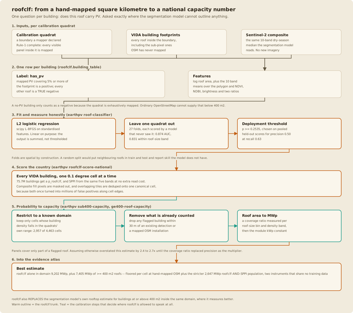
The six stages below follow the chart from top to bottom.

1. Where the labels come from, and why they have to be quadrats

Ordinary OpenStreetMap is incomplete at small sizes, so a building with no mapped PV is not a negative: it may simply be unmapped. A classifier trained on that learns to predict mapping effort rather than solar panels.

The fix is the calibration quadrat: a small area, typically 1 to 7 km², that a mapper has swept exhaustively and declared Rule-1 complete, meaning every visible panel inside the boundary is mapped. Inside such a box, and only inside it, a roof with no mapped PV is a genuine negative. That is exactly the supervision missing in the failure regime, which is why the quadrats are spent on training rather than only on after-the-fact correction.

Thirty-one quadrats now carry Rule-1, with 16,469 mapped installations between them; 30 feed the current fit (Kalat Rural is registered and Rule-1 but held out -- see Calibration quadrats).

Rule-1 is relative to the mapping imagery, not to the model's imagery

Mapping happens against JOSM's background layers (Esri, Bing, Maxar), whose capture date is generally older than the Sentinel-2 composite the model reads. A panel built between the two dates is present in the model's input and absent from the labels. So measured precision is a lower bound, base_rate is a lower bound, and rate_ratio is an upper bound. Recall over mapped installations is unaffected, since it only ever divides by labels that exist. Closing this properly needs contemporaneous high-resolution imagery; scripts/fraction_stale_label_audit.py is the interim way to bound the size of the gap.

2. One row per building

roofclf.building_table turns each quadrat into a table, one row per VIDA building whose representative point falls inside the boundary.

The label. A building is a positive (has_pv = 1) when mapped PV polygons cover at least 5% of its footprint (MIN_PV_OVERLAP_FRAC). The threshold exists so an array that merely clips a neighbour's roof edge does not label that neighbour. The true intersected area is kept as pv_area_true_m2, and it is that column, not the building's size, that later measures how much of a flagged roof the panels actually cover.

The features. Seventeen numbers, all read off the same dry-season composite the segmentation model uses. No new imagery is fetched at any point.

Block	Columns	What it carries
Size	log_roof_area, bf_confidence	the adoption propensity that comes with a bigger roof, plus the footprint's own confidence score
Reflectance	10 band means over the footprint	the roof's spectral signature, averaged over whatever real pixels it has
Derived	ndvi, ndbi, brightness, swir_vis_ratio, blue_red_ratio	vegetation and built-up contrast, and the dark, comparatively flat visible response with a SWIR drop that characterises a module

Roughly half of Pakistani VIDA footprints are smaller than one pixel and rasterise to no pixel at all. Those fall back to the pixel under their representative point, the same convention density.py uses. Without that fallback the entire small-building population, which is the population this module exists for, would drop out of the table.

Two feature blocks are computed and left switched off by default, because the ablation did not support them: footprint shape (compactness, rectangularity, aspect ratio) and the segmentation and fraction rasters as inputs. See the ablation below.

What a PV roof looks like in the spectral domain

The features above are numbers, and it is worth seeing what they actually measure. Take every sub-400 m² building in the Rule-1 quadrats, split by whether it carries mapped PV, resample the PV-free class to the same roof-size mix so nothing below is a size effect in disguise, and plot the two median spectra:

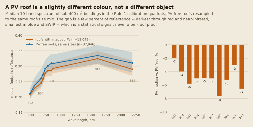
Two honest readings of that figure, and both matter:

• There is a real, physically sensible signal. A roof carrying panels reads darker in every band, because glass over silicon absorbs where a concrete or metal roof scatters. The dip is deepest in the red and near-infrared (6 to 8% from B04 through B08, which is the light a module exists to absorb) and shallowest in blue and in the first SWIR band (glass reflects blue slightly better, and silicon stops absorbing beyond its band gap, so B11 recovers to a 3% gap). That shape, "dark, slightly blue, with a relative SWIR excess", is what the derived features (blue_red_ratio, ndbi, brightness) each capture one slice of, and it is the same physics SPPI hard-codes as a formula.
• The signal is statistical, not diagnostic. The interquartile ribbons overlap almost completely: plenty of PV-free roofs are darker than the median PV roof. No band, and no threshold on any band, sorts individual buildings cleanly. That is why this instrument is a calibrated probability that gets summed into an adoption rate, never a per-roof verdict, and why everything downstream (the deployment threshold, the coverage ratio, the domain restriction) exists.

The same point, measured rather than eyeballed: each spectral cue on its own separates the two populations only weakly, and the working instruments are combinations.

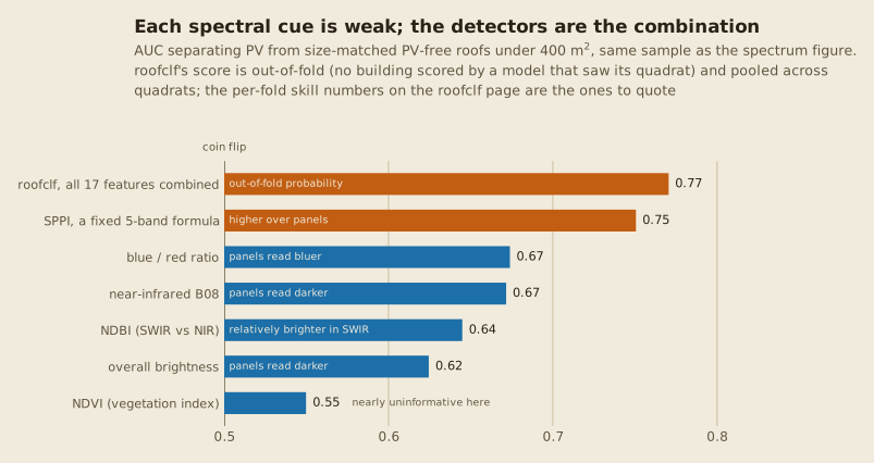
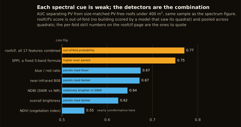
Read the levels, not the exact values: this chart pools out-of-fold scores across all quadrats and restricts to size-matched sub-400 m² buildings, which is the hardest cut and makes both combinations look closer to each other than the per-fold skill numbers below, which are the ones to quote. What the chart establishes is the ordering: a vegetation index knows almost nothing here, each single physical cue is worth a few points over chance, and stacking ten bands plus the derived ratios is what turns a tint into an instrument. Source data: results/detection_spectral_signatures.csv and results/detection_feature_auc.csv, written by scripts/detection_domain_examples.py from the quadrat building table.

The parcel label (--parcel-label, 2026-08-16)

The roof term above is the geometric intersection of mapped PV with the footprint, so an array two metres off the wall contributes exactly zero to pv_area_true_m2, and therefore zero to the coverage ratio and zero to the area recall, on a building this classifier usually flags anyway. --parcel-label closes that by adding the mapped PV that sits off every footprint but within 20 m of one, attributed wholly to its single nearest building.

Three rules stop it double-counting. Each installation has the footprints it intersects subtracted before the remainder is measured, so the roof and yard terms partition one polygon. The remainder goes to one building, not to every building in range. And anything at or above 400 m² is skipped entirely, because above that floor ground-mount belongs to segmentation and the atlas already counts it there. The 20 m ring also sits inside the 30 m radius the OSM and candidate dedup masks already use, so nothing it picks up can survive a dedup that a nearby mapped feature should have removed.

Two different things arrive in that term, and the table keeps them apart. Measured across the 27 quadrats:

Term	Area	Share of parcel PV
pv_area_roof_m2	1,763,024 m2	92.3%
pv_area_yard_ground_m2 (OSM placement=ground)	29,764 m2	1.6%
pv_area_yard_overhang_m2 (rooftop PV past its VIDA outline)	117,003 m2	6.1%

Only the middle row is the small ground-mounted PV the widening was built for. Most of what it adds is mapped rooftop PV whose polygon extends past an imagery-derived VIDA footprint, which is a real undercount in the roof-only label rather than ground-mount: VIDA outlines are routinely undersized or a metre or two off. Including it is self-consistent, because an undersized footprint shrinks the calibration denominator and the national flagged roof area by the same bias, so the ratio still transfers. But it means the resulting capacity figure is not "rooftop plus ground-mount" in the proportion the headline suggests, and both capacity summaries carry a parcel_label_composition block reporting the split for exactly that reason.

What the label costs and what it moves, both measured on the same 27 quadrats:

	roof-only	parcel
median fold AUC	0.8786	0.8735
within-size AUC	0.8342	0.8312
deployment threshold (precision 0.5)	0.2511, recall 0.634	0.2535, recall 0.633
rate_ratio-trusted quadrats	16	17
sub-400 m2 pooled coverage ratio	0.1935	0.2096
sub-400 m2 pooled area recall	0.8179	0.8041
>= 400 m2 pooled coverage ratio	0.2313	0.2303

The small AUC cost is expected rather than a regression: the parcel label is a harder target, adding 817 positives whose evidence lies partly outside the footprint the features describe. The capacity effect runs the other way, and almost entirely through the sub-400 m² half: a coverage ratio 8.3% higher divided by an area recall 1.7% lower.

Scored nationally (4,470 cells, 75.7M buildings) and run through the full capacity chain, it moves every roofclf-derived component:

Component	roof-only	parcel
sub-400 m2 central	7,890.2 MWp	9,201.7 MWp
sub-400 m2 AND-gate (the internal floor's small-PV half)	2,179.7 MWp	2,647.0 MWp
>= 400 m2 roofclf rooftop replacement	7,189.4 MWp	7,405.0 MWp
Best estimate	18,218.4 MWp	19,745.9 MWp
Best estimate 90% CI	14,346 to 21,768	16,051 to 23,520

About two thirds of the sub-400 m² move is the larger flagged population (1.24M to 1.36M buildings in-domain, since the widened label has 5% more positives and the precision-targeted threshold recalibrates to them) and one third the higher coverage ratio.

Unlike the 2026-08-15 recall correction, this one moves the internal floor too, from 5,389.5 to 5,856.8 MWp. That is intended and does not weaken the floor's meaning. The recall correction was kept out of the AND-gate tiers because it extrapolates to installations neither detector saw, which a floor may not do. The parcel label does the opposite: it prices the buildings both detectors already agree on more completely, using PV that is mapped and measured on those same parcels.

Published 2026-08-17

These are the published figures. The parcel label passed its random-cell manual validation (20 cells, seed 20260817, tiles in results/pakistan_roofclf_parcel_validation/), reviewed by the repository owner, and the calibration and national scoring were promoted to the canonical paths (data/roofclf/, data/roofclf_national_with_sppi/<aoi>/). The roof-only versions they replaced are kept alongside as *_PRE_20260817_parcel_label, so every pre-widening figure remains reproducible.

The yard feature block does not ship. yard_features computes the same statistics over the yard that the roof block computes over the footprint, partitioned by a distance-transform Voronoi so no pixel is credited to two buildings, plus SPPI, the strongest single spectral discriminator for a yard array. Against the parcel label itself it still loses to the roof-only feature set (median fold AUC 0.8712 against 0.8734, and 0.7538 for the yard block alone against a 0.7382 size-only baseline). The reason is in the table above: 80% of what the parcel label adds is rooftop PV that roof features already see, and the ground-mounted term is 1.6% of quadrat PV area, too small to move a 118,755-row fit. It stays available behind --yard-features for re-measurement once cropland quadrats exist.

3. The model, and how skill is measured

A regularised logistic regression, fitted with scipy's L-BFGS on standardised features, with an unpenalised intercept. Gradient boosting was passed over deliberately. The output is summed into an adoption rate and a capacity, not thresholded and forgotten, so it has to be a calibrated probability; and with a few tens of thousands of rows across two dozen spatial folds, a linear model in good features is the appropriate capacity. Leaving out scikit-learn also keeps this stage runnable in the base environment, with no PyTorch.

Skill is measured leave-one-quadrat-out. Every building's reported score comes from a model that never saw its quadrat. A random split would put two roofs on the same street in train and test and report skill the model does not have.

Measure	Value	Read it as
Median fold AUC	0.879	ranking skill on a quadrat the model has never seen
Median fold AUC within roof-size band	0.834	the same, with size removed as a discriminator
Segmentation raster, within size band	0.500	chance. The 400 m2 floor, measured
Fraction head, unconditional	0.634	better than segmentation, still well behind

Why the within-size number is the honest one

Adoption genuinely rises with house size: mappers report large houses packed with PV and small ones much less. A classifier handed footprint area therefore scores well above chance from that propensity alone, and in the ablation below area_only reaches 0.744 without the imagery contributing anything at all. auc_within_size scores inside roof-area bands and weights by band size, which removes size as a discriminator entirely. What is left is the pixels separating a PV roof from a PV-free roof of the same size. Quote 0.834, not 0.879.

What the pixels actually add

Leave-one-quadrat-out median AUC per feature block:

Feature block	AUC	AUC on buildings below 500 m2
Size only	0.737	0.721
Reflectance only	0.840	0.840
Size plus reflectance (shipped)	0.879	0.877
Plus footprint shape	0.878	0.876
Plus the segmentation and fraction rasters	0.878	0.870

Reflectance alone beats size alone by a wide margin, which is the result that matters: the model is reading roofs, not guessing from a size prior. The last two rows move the number by no more than about 0.001, well inside fold noise, so neither block is switched on. Adding the segmentation raster in particular has no case: it is trained with sub-400 m² arrays burned as ignore, so its probability there is noise a fit can only chase.

Folds are not one population, and should never be pooled

Skill has to be read per quadrat. Industrial estates and dense residential neighbourhoods are not the same problem, and the folds say so: the best fold reaches 0.98 (Muzaffargarh Rural Wide, 9 mapped installations) and the worst 0.66 (Khairpur Rural, a rural box with three mapped installations, where AUC is barely defined). Mardan at 0.766 is the weakest fold with a real sample behind it and is excluded by name from the capacity calibration. Nasirabad Rural, this project's first confirmed-zero-installation quadrat (see Calibration quadrats), has no AUC at all -- roofclf.auc() returns NaN by design when a fold has no positives to rank against, rather than raising.

Ranking transfers between places. Absolute rates do not.

rate_ratio, the model's predicted adoption rate divided by the true one, spans 0.28 to 4.41 across the 26 quadrats with a defined true base rate. The predicted rate is nearly flat (mean about 0.14) while the true base rate spans under 1% to over 25%, so the ratio is close to constant / base_rate by arithmetic. Any published adoption rate or capacity needs a per-stratum correction first. Everything in stage 5 exists because of this. (Nasirabad Rural's own rate_ratio is nominally in the millions -- dividing by a true base rate of exactly zero -- which is why it is excluded from this span rather than reported as if it meant something.)

4. The deployment threshold

A national scorer needs one operating point, and it is chosen for precision, not for balanced sensitivity: this signal contributes to a capacity number that no human reviews, so a false positive is expensive here in a way it is not in the mapping-leads queue.

p_roofclf >= 0.2511 is the smallest threshold holding precision at 0.50 on the pooled out-of-fold scores, and it catches 63% of PV-carrying buildings there. Both numbers are still leave-one-quadrat-out measurements: one threshold instead of 27 per-fold ones, but no building was ever scored by a model that saw its own quadrat.

The threshold moves whenever the quadrat set changes -- it has ranged from about 0.24 to 0.46 across refits as quadrats were added or dropped. Anything downstream that hard-codes it is a bug.

5. Scoring a country

earthpv roofclf-score-national applies one pooled fit, on all quadrats together, to every VIDA building in the AOI, working one 0.1 degree cell at a time, resumable per cell in the same way density.py is. For Pakistan that is about 75.7 million buildings across 4,463 cells and two to three hours on CPU. Each building gets p_roofclf and, from the same five bands at no extra read cost, an SPPI value.

Two bugs were found here that are worth knowing about, because both produced enormous, plausible-looking false-positive populations rather than crashing:

• Composite fill read as near-certain PV. A tile's bounds round-trip through lat/lon and back inflates the requested window past the tile, and the merge fills the excess with zeros. Zero reflectance is darker than any roof, and PV is dark, so an all-fill footprint scored 0.73. That was 2.86 million buildings, 45.6% of every flagged building in the country, in a band along every cell edge. Fill pixels are now excluded from the zonal statistics, and a footprint left with no valid pixel keeps its row but scores NaN, which can never clear a threshold. Full write-up: cell-edge false positives.
• The same building scored twice. Composite tiles overlap, and Pakistan's tile set carries two grid origins describing the same ground, so a building could be claimed by two differently-named cells. Cells now come from a canonical, deduplicated manifest and each reads its own exact 0.1 degree box.

6. From a probability to a capacity number

A flagged building is not yet a megawatt. Three corrections stand between them, and each one exists because skipping it produced a number that was wrong by a factor rather than by a few percent.

Restrict the domain. roofclf only counts buildings in cells whose building density falls inside the range spanned by the calibration quadrats themselves, currently 48.5 to 5,258 buildings per km². That is 2,957 of Pakistan's 4,463 cells, 66.3% of cells and 94.7% of national buildings. The restriction is the whole answer to the rate_ratio problem above: rather than correcting a rate the evidence cannot support, the module refuses to speak where no quadrat resembles the ground. Rescaling the domain figure by its share of cells or buildings to get a national total is exactly the error this design prevents, and sub400_capacity's own returned summary says so.

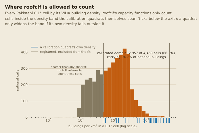
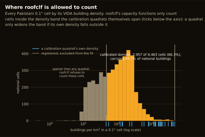
The histogram also shows why widening is hard: the out-of-domain tail is sparser than every quadrat tick, and most cells sit just left of the band's lower edge. One low-density quadrat moves the edge much further than another urban one ever could -- which is what the deliberately rural extensions below were for.

Widening the domain therefore needs new ground truth, not new code, and the constraint is subtle: a quadrat extends the range only if its own average density falls outside the current band. A boundary traced around a village, the natural way to draw one, is dense by construction no matter how empty the surrounding cell is. Two quadrats deliberately drawn to include farmland alongside a settlement took the lower edge from 553 to 141 buildings/km² and grew the domain from 646 to 1,680 cells; a third, Bahawalnagar Rural (hand-drawn in JOSM, own density 123.5 buildings/km²), pushed it down again to 1,868 cells; a fourth, Nasirabad Rural (this project's first confirmed-zero-installation quadrat, own density 48.5 buildings/km²), pushed it down again to 2,957 cells the same day. Tank Rural, added alongside Nasirabad Rural, measured 55.75 buildings/km² -- inside the widened range, but not itself the new floor.

Remove what is already counted. A flagged building within 30 m of an existing segmentation candidate, or of a mapped OpenStreetMap installation, is dropped. Anything whose own footprint is at least 400 m² is dropped from the sub-400 figure too, since that is a matching gap rather than small-PV signal. The OSM half of this was missing until 2026-08-06 and was double-counting about 3% of the capacity.

Convert area honestly. Panels cover part of a roof, not all of it. Multiplying flagged roof area by precision alone, which was the original approach, corrects for false positives and silently assumes full coverage. Measured against the quadrats' own mapped pv_area_true_m2, real coverage is about 0.19 of a flagged footprint for roofclf alone and 0.27 where roofclf and SPPI agree, so the original figures were 2.4 to 2.7 times too high. The coverage ratio is now fitted per roof-size bin and per building-density band, then 0.18 kWp per m² of module converts covered area to capacity.

The quadrat ground truth shows directly what that ratio is pricing, and why it must be fitted by size rather than pooled:

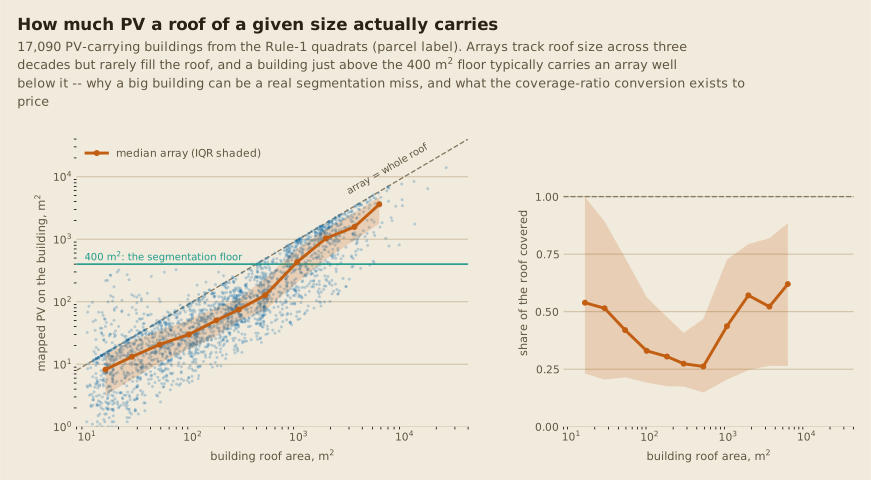
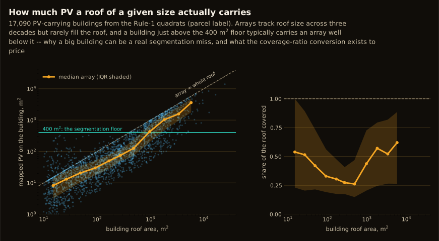
Two readings. First, the coverage share is not one number: it is U-shaped in roof size (small homes fill half the roof, mid-size buildings barely a quarter, big industrial roofs climb back up), which is exactly why the ratio is fitted per size bin. Note these medians sit above the 0.19 quoted in the previous paragraph because they are measured on buildings that truly carry PV, while the deployed ratio is measured over roofclf-flagged roofs, false flags included. Second, the left panel is the measured case for the ≥ 400 m² roofclf replacement below: a building above the floor usually carries an array below it (median 127 m² of PV on a roughly 485 m² roof), so segmentation can miss a large building's array outright without that being evidence the roof is empty.

Where the numbers land

Component	Population	MWp
Sub-400 m2, roofclf and SPPI agreeing, in domain	Internal floor on Best estimate	2,515
Sub-400 m2, roofclf alone, in domain	Best estimate	8,923
At or above 400 m2 rooftop, roofclf, in domain	Best estimate	6,747
Sub-400 m2, roofclf and SPPI agreeing, outside the domain	Not published (dropped 2026-08-15)	69

The published atlas total, which also carries hand-mapped OSM and the segmentation model's own ground-mount and out-of-domain rooftop estimates, is Best estimate 18,826.7 MWp (90% range 16,022 to 24,358) -- the first three rows only. The fourth was dropped from the published atlas on 2026-08-15 (see the last bullet below); its capacity function and CLI flag remain for anyone who wants that estimate explicitly. (Updated 2026-08-20: three peri-urban calibration quadrats -- Attock, Layyah, Lodhran, docs/issues/pakistan-calibration-boxes.md's Box 18 -- were declared Rule-1 and folded into a fresh roofclf refit, 30 quadrats total, moving every row in this table down together.)

The two Best-estimate roofclf rows are recall-corrected as of 2026-08-15: the coverage ratio prices the PV on roofs roofclf flagged, and dividing by the measured share of true mapped PV area that lands on a flagged roof (0.808 sub-400 m², 0.978 at or above 400 m², per size bin and density stratum) extends that to the roofs it missed -- the same correction the segmentation half has always used. The floor row is deliberately left uncorrected, because a floor that extrapolates to installations neither detector saw is not a floor. See the capacity map for the full derivation and the three ways the correction is a lower bound on itself.

Three things about that table are worth stating plainly:

• SPPI is a second opinion, not a feature. Adding SPPI as a roofclf input changes AUC from 0.8736 to 0.8734, which is nothing. Requiring the two to agree raises precision from 0.53 to 0.63 on the same quadrats, at 0.46 recall instead of 0.73. They share no training data, which is why agreement between them is evidence and why it sets the internal floor under the atlas's headline figure.
• At or above 400 m², roofclf replaces segmentation rather than adding to it, inside the calibrated domain only. Measured on the identical 92 cells at the time of the swap, roofclf's rooftop estimate came to 2.18 times segmentation's. Outside the domain, segmentation's own recall-corrected number stays authoritative, because it is the only evidence-backed figure there.
• The out-of-domain row is a labelled extrapolation, and is no longer published (2026-08-15). All of those cells sit below the calibrated density band, with a median density roughly six times sparser than the least dense quadrat, so a coverage ratio measured on urban quadrats was being applied to rural ground where nothing constrains it, and the JOSM pass meant to test that population could not be done: the reference imagery there is too old to confirm or refute recent installations. It fed Best estimate only, drawn with its own dotted outline; dropping it moved the headline 18,280 to 18,218 MWp (pre-parcel-label figures) and left the floor untouched. Everything the atlas now reports is measured where it is applied.

What roofclf cannot do

• Ground-mounted PV below 400 m² has no instrument at all. roofclf scores a building footprint, and a small free-standing array does not have one. This is a distinct open gap, not a smaller version of the rooftop one.
• Very bright non-PV roofs. A cluster of white-roofed buildings in cell 0061_0012 scores 0.98 to 1.00, and SPPI does not catch them either, so the AND-gate does not help. Retraining on the six known examples changed nothing, and oversampling them traded away general skill; mining more of the pattern is the open lead, and mining them through glint works only for roofs at or above 1,000 m², which is not where this failure lives.
• Exact attribution in dense clusters. In the tightest quadrats the median spacing between neighbouring small installations is 15 to 20 m, at or below one Sentinel-2 pixel. A flagged polygon there can sit among several real arrays rather than on the one carrying the panels. That is a sensor-resolution ceiling, not a training defect.
• Speak for the country. Everything above is scoped to the calibrated domain, and the restriction is enforced in code rather than left to the reader.

Running it

# 1. Fit on every discovered quadrat, evaluate leave-one-quadrat-out, pick the threshold.
pixi run earthpv roof-classifier --aoi pakistan

# 2. Score every building in the country. Long: two to three hours, CPU only, resumable.
pixi run earthpv roofclf-score-national --aoi pakistan

# 3. Essential, not optional: validate against randomly drawn cells in JOSM.
pixi run roofclf-tiles -- --random-cells 20 --seed <fresh int> --mapcss

# 4. Turn probabilities into capacity. Both are CPU only and take minutes, because the
#    domain restriction means only the matched cells are ever read.
pixi run earthpv sub400-capacity     --aoi pakistan --osm-solar <national OSM solar pull>
pixi run earthpv ge400-roof-capacity --aoi pakistan --osm-solar <national OSM solar pull>

Then rebuild the evidence atlas from the building-level parquets those two steps write: see Setup New Country steps 13 to 15 for the exact earthpv atlas invocation and its four --sub400-* / --ge400-roof-cells flags.

Quadrats are discovered from disk, so a new *_calib_*_boundary.geojson with a matching mapped-solar pull is picked up with no flag. roof-classifier writes data/roofclf/: model_full.json (the pooled fit every later step reads), buildings.geoparquet (every labelled building with its out-of-fold probability), folds.csv, ablation.csv and summary.json. Step 3 is part of the workflow rather than an extra: the quadrats are curated and industrial-leaning, so scoring well on them is not evidence that the model works on the un-curated rest of the country.

Read next

Topic	Page
The quadrats: how they are drawn, mapped and declared complete	Calibration quadrats, Quadrat protocol
The random-cell validation protocol and its log	Roofclf random-cell validation
How the sub-400 m2 capacity bracket was arrived at	Capacity density
The national deployment write-up and the temporal features that failed	Roofclf national deployment
The cell-edge and tile-overlap bugs in full	Roofclf cell-edge false positives
SPPI, the zero-training index it is cross-checked against	SPPI spectral index
Whether a complete register agrees with any of this	Validation against MaStR