PV calibration-ground mapping protocol (Pakistan)

Audience: the OSM mapping team building calibration areas for EarthPV's Sentinel-2 solar-density estimation. Status: in effect for every quadrat mapped so far; most recently amended 2026-08-11 (Rule 1's imagery-epoch bound, below).

Why this mapping exists

EarthPV estimates rooftop/ground PV density per 0.1° grid cell across Pakistan from 10 m Sentinel-2 imagery. The model is deliberately recall-first: it overcounts in some landscapes (bare/arid land looks like panels) and undercounts in others (small roofs are below sensor resolution, so detection measured at only ~6% for sub-100 m² installations vs ~73% for utility plants). To publish honest density numbers, we measure these errors against ground truth: small areas where every PV installation is mapped, so the model's output over each area can be compared against reality, per landscape type.

That works only if "no PV mapped here" genuinely means "no PV exists here." This leads to the one rule that overrides everything else:

Rule 1, completeness beats coverage. A quadrat is only usable when every visible panel inside it, as of the reference imagery available to the mapper is mapped, down to the smallest rooftop unit. A half-mapped quadrat is worse than an unmapped one, because it silently teaches the calibration that the model overcounts. If you cannot finish a quadrat, say so; it will be excluded, no harm done.

Rule 1 is bounded by imagery epoch, not just mapper effort (amended 2026-08-11). JOSM's background imagery (Esri/Bing/Maxar) is generally captured earlier than the Sentinel-2 composite the model reads, so a panel installed in that gap cannot be mapped no matter how carefully the quadrat is swept -- it exists in the model's input and cannot exist in the labels. A Rule-1 declaration therefore certifies "every visible panel as of the mapping imagery's capture date," not "there is no PV here the model could see." Record the imagery layer and its best-known capture date for every quadrat (imagery_layer/imagery_date below) so this gap is visible per-quadrat instead of assumed away.

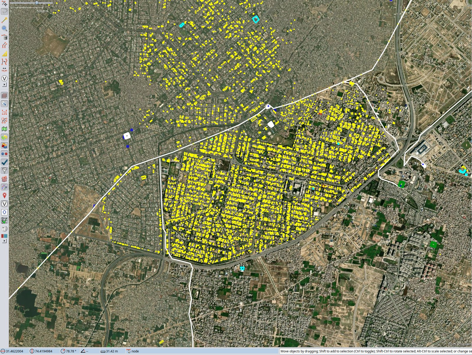
What a finished calibration area looks like, and why the boundary matters. Inside the line every visible panel is mapped; outside it nothing is, and the two look identical on imagery. This is the whole point of Rule 1: the model's output over this area can be compared against reality only because "no polygon here" genuinely means "no panel here", and that guarantee stops exactly at the boundary. Note that the boundary follows a ring road and a railway rather than being a square, which is usually the better choice.

New to JOSM? Borrow the MapYourGrid guides

MapYourGrid is Open Energy Transition's grid-mapping campaign, and its JOSM material is written for exactly this shape of work: volunteers, OpenStreetMap, JOSM, a strict quality bar. The subject is power lines rather than solar panels, so its presets and tagging do not carry over, but everything about the editor does. Rather than restate it here:

Page	What to take from it
Installation instructions	Installing JOSM on Windows, macOS (brew install --cask josm) and Linux. Start here if you have never run it.
Starter-Kit, JOSM section	Configuring the editor: presets, quality-assurance settings, custom map paint styles, the download-edit-upload loop, and a list of common beginner mistakes. The paint-style part is directly reusable, since this protocol also ships a .mapcss.
Map It	What it looks like when a campaign hands a mapper a concrete, bounded task instead of "go map somewhere". A calibration quadrat is the same idea with a harder completeness rule.
Strategies	The campaign mechanics, and the most transferable page of the four. See below.

Four of MapYourGrid's strategies map onto this protocol almost unchanged:

• The todo plugin, for working a list of objects down to zero, is how you sweep a quadrat block by block instead of roaming. Rule 1 is a completeness claim, and roaming is how a box ends up half-swept.
• Filters, to isolate one kind of object while you work. Here that is power=generator with generator:source=solar.
• fixme tags as inter-mapper communication. This protocol already uses fixme=incomplete calibration quadrat for exactly that purpose.
• Pre-upload validation and peer review. JOSM's validator before every upload, and a second mapper independently sweeping the same box, which this protocol requires as part of the completeness declaration rather than as an optional extra.

Defining calibration regions in a new country

Everything below this section is written from Pakistan's experience and uses Pakistan's landscape strata. The rules transfer; the specific strata and numbers do not. If you are bringing up a country from nothing, this section is the one to read first.

You are calibrating two different instruments, and they want different things

	roofclf (per-building, below the floor)	Segmentation (candidate polygons, above it)
What it needs	Small areas where every installation is mapped (Rule 1)	Human verdicts on a sample of the model's own candidates
Built by	this protocol	earthpv calibrate-sample then calibrate-candidates
Used for	coverage ratio, area recall, the density domain	p_real per size/placement bin, the recall correction
Without it	no sub-400 m² half at all	est_mwp_cal collapses to est_mwp_det, a precision-honest floor

Both are called "calibration" in this repository and they are not interchangeable. France has 14 exhaustively mapped communes and no candidate-precision table, so its atlas is explicitly a floor rather than an estimate. Decide up front which of the two you are buying, because the mapping effort is not shared: one wants complete coverage of small areas, the other wants verdicts spread across the size range of what the model proposed.

How many regions, and where

The binding constraint is not the count, it is the range of building density the regions span, because that range becomes the domain the capacity estimate is allowed to cover. density.CALIBRATED_BLDG_DENSITY_BY_AOI is fitted from the density of your Rule-1 regions, and every national cell outside that band is excluded from the published figure. Pakistan's 30 regions span 48.5 to 5,258 buildings/km² and that buys 66.3% of national cells, holding 94.7% of buildings. The rest of the country is not estimated.

So plan the set against your own national cell-density distribution, which earthpv density produces before any of this:

1. Compute the density distribution of the cells you intend to publish over.
2. Place regions so their own densities span it, paying particular attention to the sparse tail, which is where a set assembled by convenience will have no coverage.
3. A region only extends the domain downward if its own average density is below the current floor. A boundary traced around a settlement almost never achieves this, because villages are dense and it is the farmland between them that pulls a national average down. A range-extending region has to be sized and sited to average in unbuilt land on purpose.
4. Six to ten regions is enough to start fitting; Pakistan needed the twenties before the sparse band stopped moving. Add until the coverage ratio in your sparsest stratum stops changing when you add another.

Derive your own density band and register it. A country with no entry in CALIBRATED_BLDG_DENSITY_BY_AOI falls back to Pakistan's band with a warning that is easy to miss in a long log. Pakistan's band is meaningless in a country with different settlement patterns, and the failure is silent: you get a plausible national number covering the wrong cells.

Shape is free; size is not

A calibration region does not have to be a box. Any closed shape works, and several disjoint pieces in one file are unioned into a single region. Nothing downstream cares: chips.quadrat_chips, roofclf.building_table and every evaluation script mask and rasterise the real geometry. Following a suburb boundary, an industrial estate, a canal or the edge of the built-up area is usually better than a square, because a square clips arbitrary halves of whatever it lands on and leaves you mapping half a neighbourhood and half a field as if they were one stratum. Draw it in JOSM and hand it over with --geojson (see Drawing the boundary in JOSM).

Size has real limits, and they come from the model rather than from taste:

	Value	Why
Maximum bounding box	about 2.2 km in both directions	A training chip is 224 px at 10 m = 2,240 m. A region inside that is framed by one chip window.
Working size	1 to 4 km²	Enough installations for a stable base rate, small enough to finish.
Hard warning band	outside 0.4 to 4 km²	The importer warns and proceeds. The first Rule-1 region was 0.49 km².

Exceeding 2.24 km in either direction is allowed and loses no mapped ground, but the region is then tiled across several covering windows, which buys more training chips for the same supervision and dilutes that region's weight in the corpus. A long thin shape, say a strip following a canal for 4 km, is better registered as two or three separate regions than as one. The importer prints chip_fit and bbox_fill so this is visible before you map rather than after.

The practical floor is mapping effort, not geometry: a small region gives a noisy base_rate, a large one is a long job, and an unfinished region is worse than no region at all.

Derive your own strata, do not import Pakistan's

The six strata below are Pakistani landscape types. The transferable rule is that a stratum is a kind of place where the relationship between roofs and PV differs, and that you want several regions in each. Build the list from your own country: the split that matters is whatever changes the answer, typically some combination of building density, roof type (flat concrete behaves differently from pitched tile), urban/peri-urban/rural, and whether an area is industrial. Pick by landscape type first and look at panels second, or the sample is biased before it starts.

Reject regions on imagery date, before anyone maps

This is the single most expensive mistake in this project's history of calibration mapping, and it is now a hard gate in the tooling rather than advice.

Rule 1 certifies "every visible panel as of the mapping imagery's capture date". If that imagery predates the Sentinel-2 composite the model reads, installations exist in the model's input that cannot exist in the labels, and the region's zeros are uninterpretable in both directions: you cannot tell a real absence from an absence of evidence. Six Pakistani boxes were lost to this. Three (Dera Ghazi Khan, Waziristan, Jamshoro) were fully swept before anyone checked, and registering them would have pulled the sparse band's coverage ratio toward zero on evidence that does not support it.

So, before drawing anything:

1. In JOSM, turn on each candidate layer over the area and find its capture date. Esri World Imagery exposes dates through its own metadata; Esri Wayback and Google Earth Pro's historical slider are free ways to date a view when the layer does not say.
2. Compare it to your AOI's compose_window. If the best available imagery is substantially older, the region is not usable regardless of how much PV you can see in it.
3. Record the outcome either way:

# usable: the date goes on the boundary and travels with the region for ever
pixi run python scripts/new_calibration_quadrat.py --name sargodha_north \
    --lat 32.0836 --lon 72.6711 --side-m 1500 --country Pakistan \
    --imagery-layer "Esri World Imagery" --imagery-date 2025-03

# not usable: record it as considered and rejected, and stop
pixi run python scripts/new_calibration_quadrat.py --name dera_ghazi_khan_rural \
    --lat <lat> --lon <lon> --side-m 3000 --country Pakistan \
    --imagery-layer "Esri World Imagery" --imagery-date 2019-11 \
    --reject "imagery predates the post-2022 PV boom; zeros uninterpretable"

The script refuses to register a region without an imagery date. --imagery-unchecked overrides it and is recorded as such, so an unchecked region is visibly different from one checked and found recent. A rejection writes a row to results/calibration_rejected_regions.csv and creates nothing under data/labels/.

Record rejections, do not just abandon them. A rejection is evidence: it says someone looked here and why it was not usable. Without the register the next person re-draws the same box, and the set of regions that survives is a silent survivorship filter over wherever the imagery happened to be good, which is exactly the bias the stratification above exists to prevent.

Two siting constraints that cost this project a region

Do not site a region to include ground-mount. Kalat Rural was placed deliberately to capture a ground-mounted array, and 69 of the 89 buildings it labels as having PV are labelled only because a large ground array clips them. It is registered, Rule-1 complete, and permanently excluded from the fit. Ground-mount at or above the segmentation floor is segmentation's instrument; a roofclf region wants roofs.

A region that moves loses its purpose. Kalat Rural was sited at 25.9 buildings/km² to extend the sparse end and then moved to 46.5, where it no longer extended anything. If a region exists to reach a density band, re-check its density after any move.

Quadrat selection should be automated, and is not yet

Stated here because it is a known weakness of this protocol rather than a finished part of it. Boxes are currently chosen by hand, and two of the failure modes below are direct consequences:

• Selection bias. "Do not choose a quadrat because you already know it has solar" is a rule a human has to keep obeying. A sampler does not have to be reminded.
• Wasted mapping effort. Three boxes in Box 18 were drawn and then dropped for stale imagery, and three more (Dera Ghazi Khan, Waziristan, Jamshoro) were fully swept before the imagery date made the result uninterpretable in both directions. The imagery date is a gate that should be checked before anyone maps, not after.

What an automated selector should do: stratify by building density and landscape type from the national grid EarthPV already computes, propose boxes in the bands that are under-represented rather than the ones that are convenient, reject any candidate overlapping an existing quadrat, and check the best available imagery date for the candidate before proposing it. density.calibrated_density_range and the national cell-density table are the inputs; the density-domain lesson in Calibration quadrats is the constraint, namely that a box only widens the calibrated domain if its own average density is below the current floor, which a boundary traced around a settlement almost never achieves.

Until that exists, the manual protocol below is what is in force, and the --dry-run overlap check is the one automated guard it does have.

The quadrat plan

~25–35 quadrats across 6 landscape strata, each quadrat 1–4 km². Each stratum gets 4–6 quadrats spread across different cities/provinces; one quadrat per stratum is held out to validate the calibration and must be mapped to the same standard.

#	Stratum	Where (examples)	Quadrat size	Why it matters
1	Affluent planned housing	DHA/Bahria-type societies: Lahore, Karachi, Islamabad/Rawalpindi	1–2 km²	Highest rooftop-PV adoption; regular concrete roofs
2	Dense older urban / informal settlement	inner-city Lahore, Karachi, Faisalabad	1 km²	Small, irregular, often sub-10 m roofs, where the model undercounts most
3	Peri-urban / tehsil town	mid-size towns, one per province	2 km²	Middle of the building-size distribution, mixed roof materials
4	Irrigated rural village + fields	Punjab and Sindh canal-irrigated belts	2–4 km² incl. surrounding fields	Solar tube wells and irrigation pumps: ground-mounted, small, easily missed
5	Arid / bare-land settlement	Balochistan, Thar fringe	2–4 km²	Bare ground is the model's main false-positive class, so these measure overcounting
6	Industrial zone	Faisalabad, Sialkot, Karachi industrial estates	1–2 km²	Large metal roofs, big captive-PV arrays, different spectral behaviour

Utility-scale plants are not part of this protocol; they are already well covered in OSM and TZ-SAM.

Choosing the exact quadrat

• The boundary does not have to be a rectangle. Any closed shape works, and following roads, canals or the edge of a built-up area is usually better than a square, because a square clips arbitrary halves of whatever it lands on. See "Drawing the boundary in JOSM" below for how to hand one over.
• Snap edges to features that are unambiguous on imagery, so a second mapper can tell exactly where the boundary runs.
• Pick typical neighbourhoods, not showcase ones. Do not choose a quadrat because you already know it has (or lacks) solar. That biases the sample. Pick by landscape type first, look at panels second.
• Avoid quadrats that straddle two strata (e.g. half planned housing, half informal). Move or reshape the boundary until it is one thing. An irregular boundary makes this easier, not harder: it can follow the actual edge of the stratum instead of splitting the difference.
• Record the boundary as a GeoJSON polygon before mapping starts.

Drawing the boundary in JOSM

You can draw a calibration boundary directly in JOSM and export it as GeoJSON, which is often better than a square: it can follow a suburb, an industrial estate or a canal instead of clipping arbitrary halves of both.

Draw it on its own layer, not on the OSM data layer. That keeps the box out of the upload path entirely, which is the safest version of the never-upload rule.

1. Layers -> New Layer (Ctrl+N). This is now the active layer, and it is not connected to OpenStreetMap.
2. Turn on imagery and draw the boundary with the draw tool (keyboard A), clicking each corner. Close the way by clicking the first node again, then press Esc to end the line.
3. With that layer still active, File -> Save As... and choose GeoJSON Files (*.geojson) in the file-type dropdown. JOSM saves the whole active layer, so a layer holding only your boundary produces a clean file.
4. Hand the file to the registration script.

Keeping the boundary on its own layer also means you can leave it open and visible while you map in the OSM layer beside it.

Then hand the file over and it gets registered with:

python scripts/new_calibration_quadrat.py --name gujranwala_east \
    --geojson ~/drawn/gujranwala_east.geojson --dry-run   # inspect first
python scripts/new_calibration_quadrat.py --name gujranwala_east \
    --geojson ~/drawn/gujranwala_east.geojson             # then register

--dry-run prints the geometry report, the overlap check against every existing quadrat, and the district lookup without writing or fetching anything. The script refuses to register a boundary that overlaps an existing quadrat unless --allow-overlap is passed, because pooling overlapping quadrats double-counts the shared installations and breaks leave-one-quadrat-out fold independence (Boxes 9 and 10 share a corner, which is why that check exists).

Or: generate the boundary with EarthPV first, then map it

The other direction, and the one to prefer when you are filling a gap in the stratum table rather than following a feature on the ground. EarthPV draws the box, you map inside it. The square is geodesic (pyproj.Geod.fwd), never drawn by eye, so its area is exactly what it claims:

# 1. look before you write: geometry report, overlap check, district lookup, no files
pixi run python scripts/new_calibration_quadrat.py --name sargodha_north \
    --lat 32.0836 --lon 72.6711 --side-m 1500 --dry-run

# 2. register it: writes the boundary and pulls live OSM solar for the box
pixi run python scripts/new_calibration_quadrat.py --name sargodha_north \
    --lat 32.0836 --lon 72.6711 --side-m 1500

That writes, into data/labels/:

File	What it is
<name>_calib_<size>_boundary.geojson	The boundary. This is the file you open in JOSM.
<name>_calib_<size>_boundary.parquet	The same geometry for the pipeline.
<name>_calib_<size>_overpass_solar.parquet	What OSM already has inside the box, at pull time.

The _calib_ in the name is load-bearing: roofclf.discover_quadrats globs for it, so a stem without it is invisible to earthpv roof-classifier and fails with "No calibration quadrats found" seconds after launch.

Do the --dry-run first, every time. It is the only thing standing between you and a box that overlaps an existing quadrat, which silently double-counts the shared installations and breaks leave-one-quadrat-out fold independence. The script refuses on an overlap unless --allow-overlap is passed; --dry-run lets you see it before the Overpass pull rather than after.

Loading a single quadrat boundary into JOSM

1. File -> Open data/labels/<stem>_boundary.geojson. It arrives as its own data layer.
2. Download OSM data for the same area (File -> Download from OSM, or Ctrl+Shift+D) into a separate layer.
3. Turn on imagery and start sweeping. See Imagery below, because which layer you are on determines what you can see.

Never upload the boundary layer

The box is not an OpenStreetMap feature. Uploading it adds a nonsense square to the map. Keep it as its own layer, make every edit in the OSM layer, and check the upload dialog's layer name before you confirm. This is the single easiest mistake to make in this workflow.

Four things about a drawn boundary that are worth knowing before you map, not after:

• Close the way. JOSM exports a closed way as a GeoJSON polygon only when it carries area tags; an untagged closed way comes out as a LineString. The importer converts a closed LineString back to a polygon and rejects an open one with a clear error, so either is fine, but an unclosed way is not.
• Several pieces are allowed. Multiple features in one file are unioned into one boundary. Every stage reads the union, so a two-part quadrat is a single unit for base rate, packing distance and leave-one-quadrat-out folds.
• Keep the bounding box under about 2.2 km in both directions. A training chip is 224 px at 10 m = 2,240 m, so a boundary that fits inside one is framed by one chip window. A larger one is tiled across several covering windows, which works and loses no mapped ground, but it buys more chips for the same supervision and dilutes the quadrat's weight in the training corpus. A long thin shape following a canal for 4 km is better registered as two or three separate quadrats. The importer prints chip_fit and bbox_fill so this is visible up front, and earthpv quadrat-chips logs the covered share of every boundary rather than truncating one silently.
• Size guidance is 1-4 km², and it is guidance. The importer warns outside 0.4-4 km² and proceeds; the first Rule-1-complete quadrat is 0.49 km². A small box gives a noisy base_rate, a large one is a long mapping job.

Nothing downstream cares about the shape: chips.quadrat_chips, roofclf.building_table and every quadrat evaluation script mask and rasterise the real geometry. What is shape-dependent is the reported side_m, which is written only for actual squares, and the _calib_<tag> name suffix, which becomes the geodesic area (..._calib_1p24km2) instead of a side length.

What counts as PV (map all of it)

• Rooftop panels of any size, including single-panel household units.
• Ground-mounted arrays of any size, in fields, yards, compounds.
• Solar water pumps / tube-well installations (panels on frames near wells).
• Solar street lights and telecom-site panels only if panel area is discernible on imagery; a lone pole-top panel smaller than ~1 m² may be skipped, consistently.
• Panels under construction: map if panels are physically visible on the imagery date.

Not PV: solar water heaters (tubes/tanks, usually round or with a visible cylinder), skylights, blue-painted roofs, water tanks. When genuinely undecidable at maximum zoom, tag with fixme=possible solar rather than guessing either way.

How to draw

• Trace the panel area only, never the whole roof. The model estimates panel area; a roof-sized polygon inflates ground truth.
• One polygon per contiguous panel group. Separate groups on the same roof = separate polygons.
• For tiny installations where tracing is hopeless (< ~4 m²), a node with the correct tags is acceptable; note panel:area in m² if estimable.

Tags

power=generator
generator:source=solar
generator:method=photovoltaic
generator:output:electricity=yes        (add value in kW only if known, never guessed)
location=roof                           (rooftop) | omit for ground-mounted

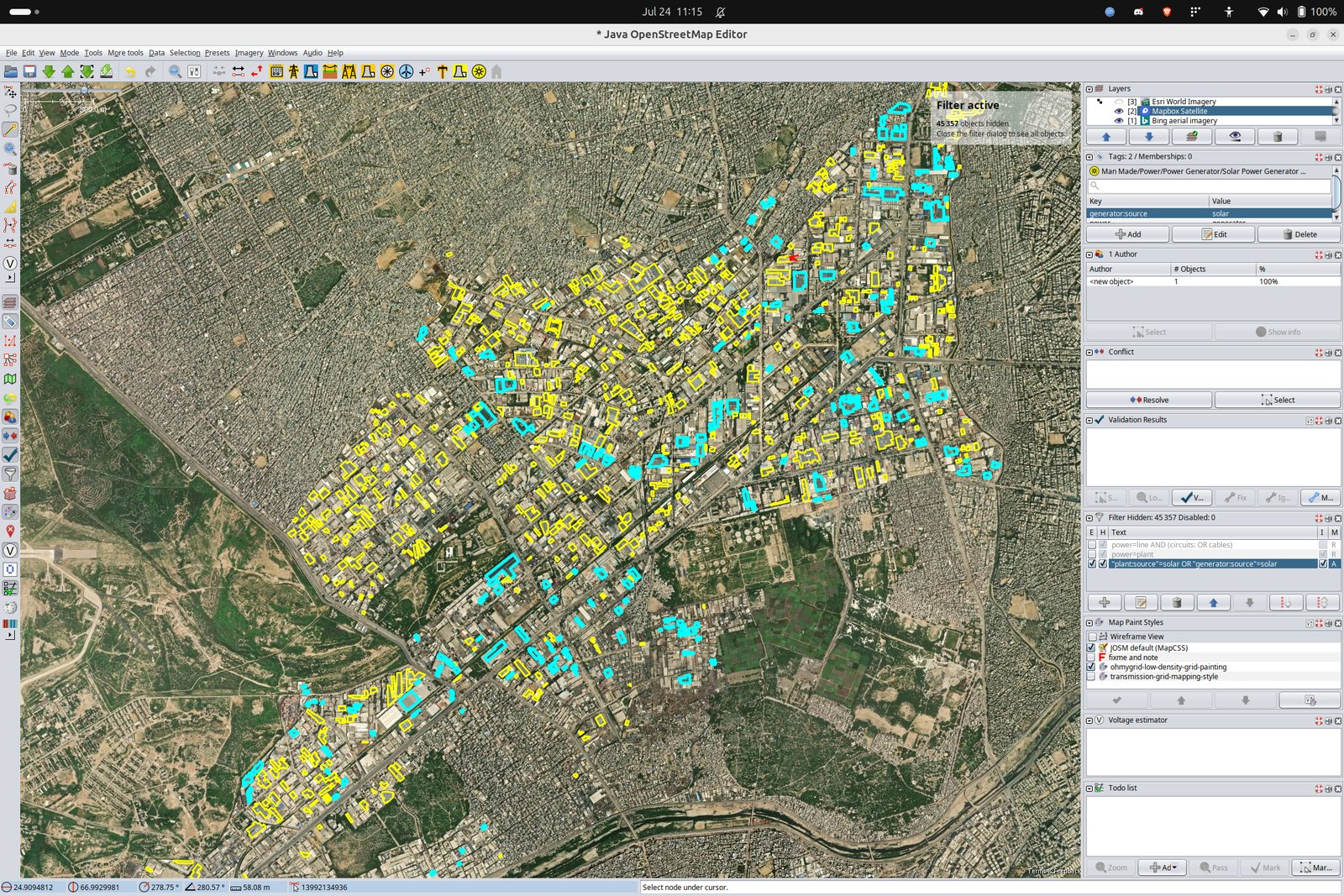
Tagging in practice, in SITE Karachi. The preset (Man Made / Power / Power Generator / Solar Power Generator) fills the tags in the table above, so they do not have to be typed by hand. The active background here is Mapbox where the previous screenshot used Esri: that switch is routine, not exceptional.

For solar pumps add pump=powered on the associated well/pump node where one exists. Do not invent capacity values; panel geometry is the ground truth here, not wattage.

Imagery and dating (critical)

• Map against the most recent high-resolution imagery available (Esri Clear/Maxar/Bing. Record which, and its capture date if the layer exposes it).
• PV in Pakistan grows fast. A calibration quadrat mapped against year-old imagery reads as "model overcounts" when the model simply sees newer panels. If the best imagery is older than ~12 months, flag the quadrat.
• Record for every quadrat: mapper name, mapping completion date, imagery layer + capture date (or "unknown").

Flip between imagery layers. This is not optional

A rooftop array that is invisible on one layer is often obvious on the next. The layers differ in capture date, sun angle, resolution and compression, and panels are a dark, low-contrast, specular target: one layer may show a flat dark rectangle, another may catch the array mid-glint as a bright patch, a third may have been flown before it was installed. Mapping a quadrat against a single background is the most common reason a "complete" box turns out not to be.

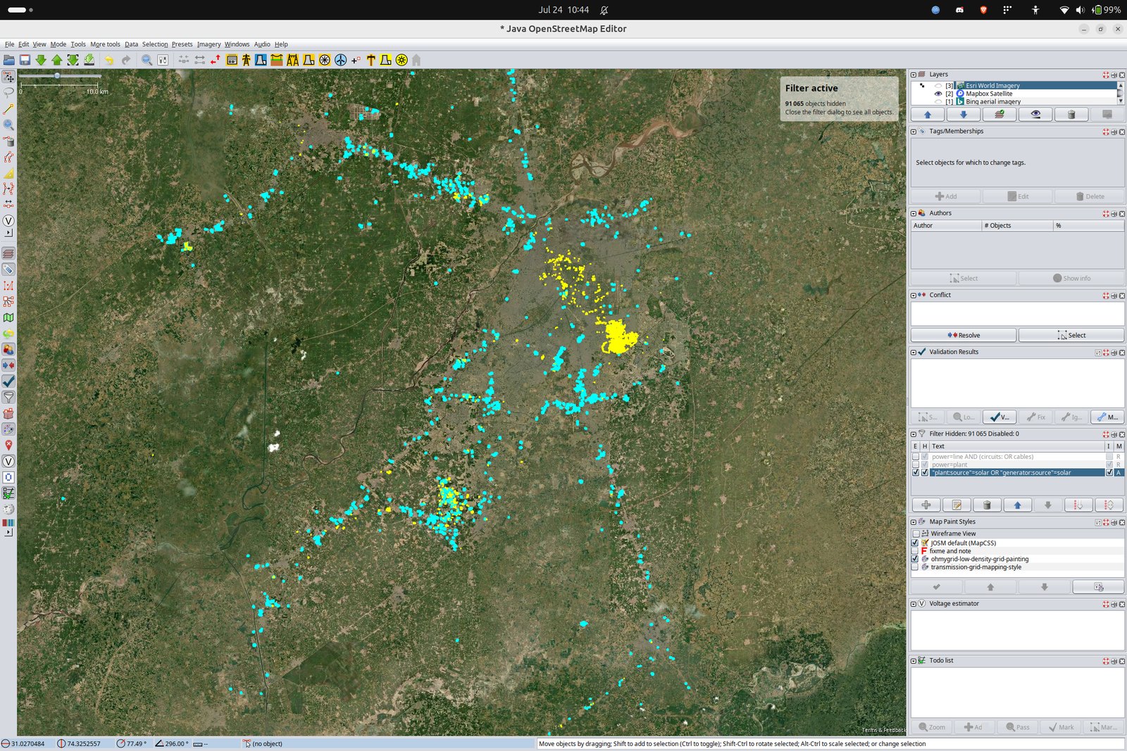
Three background layers loaded at once, which is the setup to work in: switching between Esri, Mapbox and Bing over the same roof is how you find arrays that one capture missed. The panel on the right also shows the filter doing the other half of the job, hiding 91,065 objects so that only solar-tagged features remain on screen.

Work through what your area actually offers. In JOSM these live under Imagery, and the list is driven by the Editor Layer Index, so it varies by location and changes over time:

• Bing Aerial Imagery and Esri World Imagery, the two general-purpose global layers, usually with different capture dates in the same place.
• Esri World Imagery (Clarity), often a different and sometimes sharper capture of the same ground.
• Mapbox Satellite, a third independent composite.

Toggle between them over the same roof before deciding there is no panel there. Where an installation is visible on one layer only, map it and record which layer showed it.

Many countries have national or regional imagery that beats all of the above, and it is frequently both higher resolution and more recent: national ortho services appear in JOSM's imagery list for a good number of countries in Europe, North America, Japan and elsewhere. If you are mapping in one of those, check the Imagery menu for a country-specific layer before falling back on the global ones. Two cautions: only use layers that are actually cleared for OpenStreetMap use (JOSM's built-in list is curated for this, an arbitrary WMS you add yourself is not), and read the layer's attribution requirements.

Imagery layers are frequently offset from each other, sometimes by several metres. When you flip layers, buildings appearing to move is the imagery shifting, not the OSM data being wrong. Align the imagery to existing OSM data (JOSM's imagery offset tool), never drag OSM data to match a misaligned layer, and set the offset per layer.

Known gap: imagery_layer and imagery_date have not actually been populated for any real quadrat mapped so far, even though results/calibration_quadrats.csv carries both columns. This is what makes the Rule 1 amendment above a bound rather than a correction: precision measured against these negatives, and base_rate, are lower bounds, and rate_ratio an upper bound (recall over mapped installations is unaffected), and scripts/fraction_stale_label_audit.py measures the size of that effect without any new mapping -- large in exactly the dense small-rooftop quadrats the sub-400 m² work depends on (68.4% of apparent false positives in Karachi coastal). Closing it needs imagery contemporaneous with the Sentinel-2 composite, which JOSM's default background layers do not reliably provide. See Open questions (ground-truth completeness) for the current count and cost to close it, and Calibration quadrat imagery dating for free tools (Esri Wayback, Google Earth Pro's historical slider) that could backfill it.

Uploading to OpenStreetMap

The panels you map go into OpenStreetMap itself, not into a private file. That is deliberate: the calibration needs them, and the map benefits from them independently of this project. It also means the usual OSM norms apply, and that a sloppy upload is a problem for other people rather than just for us.

Before you press upload:

• Check which layer you are uploading. It must be the OSM data layer, never the quadrat boundary layer and never the all-quadrats validation layer.
• Run JOSM's validator (Ctrl+Shift+V) and fix what it flags. Overlapping ways and untagged geometry are the usual complaints on a panel-tracing session.
• Write a real changeset comment, for example Map rooftop and ground-mounted solar PV in <place> (earthpv calibration area).
• Set the source. Put the imagery you actually traced from in the changeset source tag, e.g. source=Esri World Imagery. If you flipped between layers, name the one the geometry came from.
• Upload in reasonable chunks. A quadrat sweep can produce hundreds of features; a single enormous changeset is harder for anyone to review or revert.

If you stop partway, tag the unfinished work fixme=incomplete calibration quadrat immediately and say so in the register. An unfinished quadrat that looks finished is the one error this process cannot detect later.

After uploading, refresh the box's snapshot so the pipeline sees your work:

pixi run python scripts/new_calibration_quadrat.py --name <same name> ... # re-pull, or
pixi run calib-export                                                    # re-export all

Completeness declaration and QA

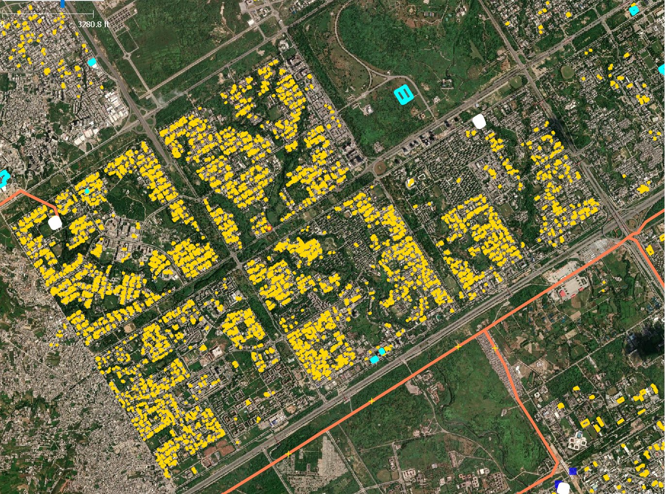
What "every visible panel" means in a residential stratum: near-total adoption, mapped house by house across whole blocks. A sweep that stopped at the large or obvious installations would have produced a fraction of this and would have taught the calibration that the model overcounts.

A quadrat is done when:

1. The mapper declares: "every visible PV installation inside the boundary is mapped": scanned systematically (street-by-street / block-by-block, not free roaming).
2. A second mapper independently sweeps the same quadrat and either adds what was missed or countersigns. Disagreements resolved together; the number of installations added by the second pass is recorded (it is itself a useful completeness statistic).
3. The declaration row is added to the shared register:

quadrat_id, stratum, province, boundary_geojson, mapper1, mapper2,
date_completed, imagery_layer, imagery_date, n_installations,
n_added_by_second_pass, notes

Packing distance is computed automatically, not recorded by hand. Once a quadrat's installations are mapped, roofclf.packing_density derives the median distance from each sub-400 m² installation to its nearest neighbour -- measured to correlate strongly (r=0.70-0.82) with how a quadrat's calibration numbers (exp_scale, auc_within_size) behave, a continuous proxy for the stratum table above (see Capacity density). Worth checking when choosing a new quadrat's location. As of 2026-07-29 the existing nine split cleanly into "packed tighter than one Sentinel-2 pixel" (7-19 m) and "sparse" (44-52 m) with nothing in between, and this paragraph called a quadrat landing in that 20-40 m gap new information rather than a duplicate. Two have since landed there -- Rahim Yar Khan at 20.3 m and Peshawar West at 34.0 m -- so the gap is now known to be an artifact of which boxes had been picked, not a real feature of Pakistani settlement. The useful check today is therefore the reverse: prefer a location whose likely packing distance is under-represented across the current thirteen, rather than assuming any particular band is empty.

Validating every quadrat in one pass

Rule 1 is judged per quadrat against high-res imagery, and doing that one boundary file at a time is how quadrats end up half-checked. This exports all of them as a single JOSM layer:

pixi run calib-export
# -> results/calibration_quadrats_validation.geojson   (every registered quadrat's
#    boundary plus its mapped installations)
# -> results/calibration_quadrats_validation.mapcss    (JOSM paint style)

Re-run it whenever a quadrat is added or an _overpass_solar pull is refreshed; it reads whatever is on disk (roofclf.discover_quadrats plus _newest_solar's dated-file-wins rule), so it never shows a stale pull. --boundaries-only drops the solar polygons if you only want the boxes; --no-mapcss skips the style file.

The layer holds two kinds of feature, and both are needed for the job. The quadrat_boundary polygon is the exact geodesic box, drawn as a heavy dashed outline with almost no fill so imagery reads through it -- completeness is judged strictly inside that line, and a panel one metre outside is out of scope rather than a miss. The mapped_solar polygons are what OSM already has, so what you are hunting is panels in the imagery with no polygon on them.

Loading it in JOSM

1. File -> Open the .geojson. It arrives as its own data layer.
2. Preferences -> Map Paint Styles -> + and point at the .mapcss next to it. Without it JOSM paints every imported way the same colour and the boundary stops being distinguishable from the panels, which defeats the point.
3. Turn on the imagery layer the register records for that quadrat (see Imagery and dating) -- not whatever loads by default.
4. Download OSM data for the box you are working on, then make every edit in the OSM layer, never in the imported one.

The style encodes what to look at:

appearance	meaning
red dashed box	quadrat boundary, Rule-1 complete
orange dashed box	quadrat boundary, not completeness-checked -- these are the ones worth your time
blue fill	mapped installation below 400 m², the population most often missing from OSM
amber fill	mapped installation at or above 400 m²
violet fill	mapped, but only partly inside the box (see below)
dashed outline	ground-mounted rather than rooftop

Never upload this layer to OSM

The boxes are not OSM features and the solar polygons are a snapshot copy of features that already exist. Uploading the layer would duplicate every installation in it and add 13 nonsense squares. Every feature carries a do_not_upload tag as a tripwire, but the real protection is keeping it as a separate layer and editing only in the OSM one.

Two things in the file that are easy to misread

Violet "edge straddling" polygons are already mapped. An installation whose representative point falls outside the box but whose footprint reaches inside is out of scope for the completeness count, yet it is still exported -- because a panel visibly inside the line with nothing drawn on it reads as unmapped, and re-mapping it would duplicate an existing OSM feature. Each box carries both counts: n_mapped_solar (all installations in the pull, the number the overview table reports) and n_inside_box.

A missing placement tag does not mean "not a rooftop". Five of the pulls (Faisalabad, Lahore, Multan, SITE Karachi, Sundar -- the oldest five) predate placement classification and carry no placement at all, so their polygons never render with the ground-mount dashes regardless of what they are. Absent, not "rooftop".

Deliverables per quadrat

• Boundary polygon (GeoJSON, in the shared register).
• All PV features mapped directly in OSM (they benefit the map as well as the calibration, and that is deliberate).
• The register row above.

Common failure modes (please read)

• Mapping only the obvious or large installations and moving on. Breaks Rule 1.
• Tracing roofs instead of panels. Inflates area ground truth.
• Choosing a quadrat because it is full of solar. Biases density upward.
• Copy-pasting a capacity guess into generator:output:electricity. Poisons downstream capacity estimates; geometry only, unless documented.
• Silent partial work: an unfinished quadrat left looking finished is the one error we cannot detect later. Mark unfinished work fixme=incomplete calibration quadrat immediately.