Capacity density

The density stage answers a different question from the detector. Instead of "where is each array", it asks "how much photovoltaic capacity is on this building, in this grid cell, in this district". That is the quantity an energy-system model consumes, and it is the only defensible way to account for installations below the per-object detection floor.

It reuses artifacts already on disk (probability rasters, candidates.parquet, VIDA footprints). No GPU, no retraining, roughly two hours single-process for all of Pakistan, resumable per cell.

Why there are four metrics

The detector is deliberately recall-first, so no single number is unconditionally honest. Each metric states its own bias.

Detected (*_det) is the area of thresholded, merged candidate polygons lying on the footprint, taken at face value. It has raw-candidate floor semantics: it includes false positives and is blind to everything below threshold, which in practice means it is blind to most residential PV.

Calibrated (*_cal) is the same area with each candidate weighted by a measured P(real | size, glint). This is the headline capacity number. It equals *_det when no calibration table exists, and it remains dependent on the 0.3 polygonization threshold.

Recall-corrected (*_rc, cell and region level only) divides the calibrated candidate area by the model's measured recall in that size bin, floored at 0.05. That is a Horvitz-Thompson estimate of the whole population at or above the detection floor, missed installations included, with 90% credible bands propagated from the calibration posteriors.

Expected (*_exp) is probability-weighted area: the sum over the footprint of per-pixel probability times 100 m², above a small noise floor. It integrates sub-threshold signal and is an upper-leaning ceiling, because false-positive probability mass gets summed too.

The chain from detected to recall-corrected, worked on one real candidate with its own bin's measured corrections:

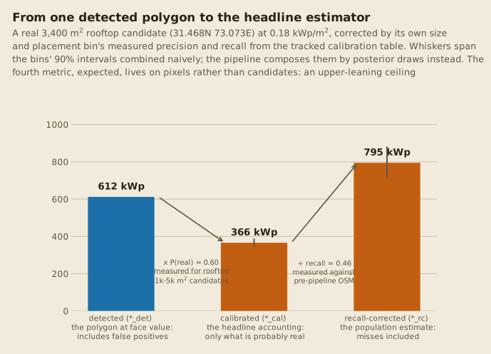
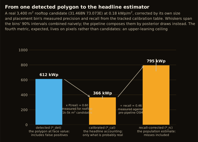
Both corrections come from the same tracked calibration table, and neither is a fudge factor: the first divides the candidate population into what is probably real, the second scales the survivors up to stand for the installations the model verifiably misses at that size. The two run in opposite directions on purpose -- a pipeline whose corrections only ever raised the number would deserve suspicion.

Reading the recall correction correctly

*_rc lives on the candidate population, so it is comparable to the *_total columns, not to the footprint-intersected *_roof ones. There is no per-building version, because the missed installations sit on other, unknown buildings. Two honesty caveats: the recall reference skews toward visible, mappable installations, which makes recall optimistic and the correction conservative; and a mapped installation counts as detected if any candidate lies within 100 m, which is generous in dense clusters. The two biases partially offset.

Area is not capacity until you know how it was mounted

Detected area means two different things depending on where the array sits, so the stage carries two conversion constants rather than one.

A rooftop detection outlines the panel field on a roof, which is close to module area: about 5.5 m² of crystalline silicon per kWp, so 0.18 kWp per m². earthpv pv-yield grounds that figure against pvlib's CEC datasheet database.

A ground-mount detection outlines the site, not the modules. The ground-PV training labels are OpenStreetMap power=plant perimeters, which enclose access roads, inter-row spacing and substations, so the model is taught to fill the fence line. Only the ground-cover ratio of that polygon is module -- 0.05 kWp per m² of site, calibrated against two named-plant ground-mount boxes (docs/issues/pakistan-calibration-boxes.md) rather than reasoned from a GCR assumption alone: Quaid-e-Azam Solar Park (400 MW / 8,904,839 m² dissolved OSM footprint) implies 0.0449 kWp/m², the Sukkur solar farm (150 MW combined, three phases / 2,606,013 m²) implies 0.0576 -- geometric mean 0.0509, rounded to 0.05. Converting site area at the rooftop constant would overstate ground-mount capacity by roughly 3.5 to 4 times.

Every all-PV estimator is therefore split by placement before conversion, and both constants carry lognormal priors (90 percent ranges of 0.15 to 0.21 for the module constant and 0.035 to 0.075 for the land constant, kept wide since n=2 real plants does not support a tight posterior and other sites plausibly use tracking or different row spacing) so the conversion propagates into the credible intervals instead of being treated as exact.

Blobs are excluded, not converted

The polygonizer merges every touching thresholded pixel with no upper bound, so a connected sheet of false positives -- a dry riverbed, salt flat, bare rock, snow -- becomes a single multi-square-kilometre "installation" whose confidence is the maximum over millions of pixels, which is to say 1.0. On the Pakistan country run 167 candidates exceeded 100,000 m² and carried 47 percent of all candidate area; the ten largest carried 27 percent, so the national total was effectively a handful of objects.

Candidates above that size are excluded from capacity. They are only flagged in candidates.parquet, so they survive in the mapping leads, where a human validates every candidate and a coarse polygon is still a usable lead. The density stage is what drops them, because it has no human in the loop. Set --max-candidate-m2 0 to disable the filter, and note that the per-building layer only reflects it after a --force rebuild; meta.json records oversize_stale_partials when it does not.

The recall curve

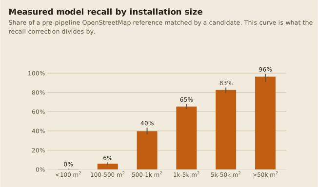
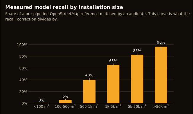
Recall is measured, not assumed: it is the fraction of installations in a pipeline-independent mapped reference that any candidate matched within 100 m. The reference is deliberately a pre-pipeline OpenStreetMap snapshot rather than a fresh Overpass pull, because a fresh pull would contain this pipeline's own validated leads and would confirm its recall upward.

The area-dominant bins above 5,000 m² are already nearly fully recalled, which is why the national recall correction adds a modest amount over the calibrated total rather than transforming it.

Outputs

Three layers plus an atlas land in data/predictions/<aoi>/density/:

File	Grain	Contents
buildings.geoparquet	building	roof_area_m2, pv_area_{det,cal,exp}_m2, pv_ratio_{det,exp}, est_kwp_{det,cal,exp}, pv_placement, region and district
grid.geoparquet, grid.csv	0.1 degree cell	roof and PV area, densities in m2 per km2, est_mwp_{det,cal,exp}, est_mwp_rc with _lo, _hi and its _roof / _ground split
regions.geoparquet, .csv, .geojson	province, or ADM2	additive totals, ratios recomputed from sums, bands re-derived from summed draws
plausibility.csv	province	the gate's per-region verdict, see below
<aoi>_pv_atlas.html	country	the self-contained interactive capacity atlas

Rooftop capacity is est_kwp = pv_area x --kwp-per-m2-module (default 0.18); the ground-mount part of every all-PV column uses --kwp-per-m2-land (default 0.05). The *_roof and *_ground columns are exported separately so the split is auditable rather than buried in a total.

Double counting is prevented at the source. Adjacent rasters overlap by a few pixels, so each building is assigned to exactly one cell by its representative point, and each cell's raster sum is cropped to the canonical 0.1 degree box.

buildings.geoparquet's rooftop sum is not the region total's rooftop component

These are two different accounting methods over the same candidates, and they are not expected to agree. The region/national rooftop total (est_mwp_rc_roof, pv_area_det_roofcand_m2 in grid.geoparquet/meta.json) sums each rooftop-placed candidate's full polygon area, exactly once. buildings.geoparquet's per-building pv_area_det_m2 instead sums, for each building, only the geometric intersection between it and every candidate that touches it (density.per_building_detected), capped at that building's own roof area. Whatever part of a rooftop-classified candidate's own polygon does not sit on any building -- gaps between the buildings it spans, general polygonize-and-merge over-draw beyond a roof's edge -- is counted in the first total and silently absent from the second.

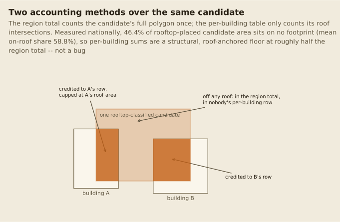
This is not a rounding difference: of 21,506,014 m² of rooftop-placed candidate area nationally, only 11,527,028 m² (53.6%) is attributed to any building in buildings.geoparquet -- a 46.4% gap (9,978,986 m²). The mechanism is exactly what it looks like: postprocess._join_buildings_metric only requires >= 30% of a candidate's own area to sit on some building before calling it rooftop (NEAR_BUILDING_M's sibling threshold), and the mean building_overlap_frac across rooftop-classified candidates is only 58.8% -- multiplying that shortfall through (sum(area * (1 - overlap_frac))) predicts a 9,781,295 m² gap, matching the measured figure to within 2%. Ground-mount is not involved: both sides of this comparison are already restricted to placement == "rooftop" candidates before summing.

Practical consequence: buildings.geoparquet's summed rooftop capacity understates the region/national rooftop total by roughly half, structurally, not as a bug to patch -- the per-building table is answering "how much PV sits on this specific building," which is a stricter and smaller question than "how much rooftop-placed candidate area exists in this region." Any PyPSA-style per-building disaggregation built from buildings.geoparquet should be read as a conservative, roof-anchored floor, not as a decomposition that sums back to grid.geoparquet's own est_mwp_rc_roof. A building_overlap_frac above 1.0 was also observed on a handful of candidates (VIDA building footprints occasionally overlap each other, double-counting a candidate's own intersection area across two overlapping buildings) -- a minor, secondary data-quality note, not the driver of the gap above.

Province polygons come from geoBoundaries (open, CC-BY), because Overture's divisions endpoint times out from the development machine. Override with --regions-file.

Completeness confidence (segmentation runs only)

Every estimator on this page (det/cal/exp/rc) is floored at >= 400 m² and its recall correction was measured on hand-mapped calibration quadrats currently spanning 553-5,258 buildings/km². Outside that settlement-density range there is no calibration evidence either way -- not "the estimate is worse there", just "untested". A segmentation density run therefore carries a density_confidence column on grid.csv/regions.csv (values below_calibrated_range / in_calibrated_range / above_calibrated_range, alongside the raw bldg_density_km2), plus n_cells_{below,in,above}_calibrated_density in meta.json. It is a flag, not a correction -- it changes no number, it only tells a reader which totals rest on measured ground and which do not (most of rural Pakistan is below the range, since every calibration quadrat is an urban or peri-urban box).

This column is deliberately computed only when exp_source == "segmentation" -- a fraction-head run is a different instrument with its own (separately tracked) calibration gaps, and sharing one flag across both would imply a validation that was never done for the one that didn't get it.

Below the detection floor: change the unit of prediction

The recall correction has a hard limit that no amount of better calibration reaches. It scales up what was detected, so 1/recall x ~0 is still ~0. Measured on the Pakistan run, the entire sub-500 m² class contributes 8.2 MWp to the national estimate, about 0.2 percent of the rooftop total, while a single exhaustively mapped square kilometre of residential Lahore holds 3.3 times more sub-100 m² PV area than the model finds in all of Pakistan. That is not a coefficient problem. A size class the detector never sees cannot be recovered by reweighting the classes it does see.

Two instruments address it, and both drop the polygon.

Expected area from a fraction head

density --fraction-prob-dir <run>/prob swaps the expected-area instrument from segmentation class probability to a fraction head's per-pixel PV coverage. This matters because the segmentation model is trained with everything below chips.MIN_PV_AREA burned as ignore, so it has no reason to put probability mass on a small array, whereas the fraction head is trained on OpenStreetMap polygons burned at 10x supersampling with no size floor.

Measured on all nine registered quadrats (earthpv roof-classifier, updated 2026-07-29 to include the three owner-mapped boxes added that day), as predicted PV area over their buildings divided by the exhaustively mapped truth (data/roofclf/exp_scale_anchor.csv):

quadrat	stratum	segmentation	fraction head
Karachi DHA 5 coastal (Rule-1)	1, coastal residential	0.000	0.042
Mardan (Sheikh Maltoon Town)	⅓, planned housing	0.000	0.196
Quetta City	5, arid/bare-land	0.256	0.204
Lahore DHA (residential)	1, affluent planned	0.023	0.520
Sialkot Old City	2, dense informal urban	0.000	0.840
Multan Industrial	6, industrial	1.710	1.350
SITE Karachi	6, industrial	2.117	1.636
Sundar Industrial	6, industrial	1.265	1.439
Faisalabad PSIE	6, industrial	1.832	2.077

Read the top row first. In the Rule-1-complete coastal quadrat, where the median installation is 86 m², the segmentation instrument predicts 0.0 m² against 13,964 m² of mapped PV -- not an underestimate, a total blank -- and the fraction head recovers 4.2 percent. In Lahore DHA, where installations are larger, segmentation recovers 2.3 percent and the fraction head 52 percent. In the industrial quadrats both run high. So the fraction head is strictly better than segmentation below the floor and by a wide margin, but its own sensitivity still collapses as installations approach 100 m²: it is an improvement, not a solution.

--exp-scale divides by a measured over-prediction factor -- still not applied nationally, and the three new quadrats reinforce rather than resolve why. The fraction-head scale now spans 0.042 to 2.077 across nine quadrats, a 49x range, and it does not collapse to a clean stratum split either: within the five non-industrial quadrats alone (Karachi coastal, Mardan, Quetta, Lahore, Sialkot) the scale still spans 0.042-0.840, a 20x range, without an obvious relationship to median installation size (Sialkot's 63.7 m² median scales at 0.840, close to Lahore's mixed-size 0.520, while Karachi coastal's broadly similar 86 m² median scales at 0.042 -- 20x lower). The four industrial quadrats are the one internally consistent group, all landing at 1.35-2.08. Averaging across all nine (mean 0.92, median 0.84) would produce a single constant that under-corrects the industrial quadrats by roughly 1.5-2x and over-corrects Karachi coastal and Mardan by roughly 5-20x in the opposite direction -- actively worse than the current uncorrected default for those strata. The default therefore stays --exp-scale 1.0. A defensible correction needs either a per-stratum multiplier (which density.py does not currently have a mechanism to apply -- there is no per-cell/per-building stratum label at that stage) or enough quadrats per stratum to fit one reliably; five non-industrial quadrats is not yet that. Germany's MaStR bench cannot settle it either, since its two slope estimators disagree by 2.6x and its well-mapped subset by 13x. These quadrats can, because their denominator is complete by construction -- there just aren't enough of them yet, especially outside the industrial stratum.

Full coverage reached; the Gilgit-Baltistan regression is exempted, but promotion still failed for a different reason (updated 2026-07-30)

As of 2026-07-29 the fraction-head run covers all 4,463 manifest cells (exp_coverage_frac: 1.0) -- the inference finished on 2026-07-27, the docs simply hadn't been updated. National expected-area rooftop capacity with the fraction instrument comes out at 6.65 GWp vs the segmentation instrument's 5.4 GWp (+23%), consistent in direction and rough magnitude with the quadrat-level finding above that segmentation is structurally blind below the floor. That comparison is architecturally clean: the exp/fraction swap touches only pv_area_exp/est_mwp_exp, nothing else in the pipeline.

The Gilgit-Baltistan ground-mount regression that originally blocked this (110 MWp against 0.000 MWp rooftop) was traced to a density.py/postprocess.py no_building-aggregation issue independent of the fraction head, and is now exempted at the region level (RATIO_CHECK_EXEMPT_REGIONS, see the plausibility gate section below) -- check-density passes again on that specific failure mode.

That exemption was not enough: promoting the fraction head as density.py's default, attempted 2026-07-30 against the current (post-OSM-replace) candidate population, failed check-density again, for a different reason. Two regions (Khyber Pakhtunkhwa, Balochistan) failed the ground:rooftop ratio check that had previously passed. Root cause: a disproportionate 46% collapse in roof-intersected candidate area vs. 29% overall between the passing baseline and the forced recompute -- the same class of density.py aggregation issue as the Gilgit-Baltistan case, now surfaced more broadly because this was the first forced full recompute combining OSM-geometry-replacement's candidate corrections with a genuine forced recompute (earlier comparison runs had pinned the candidate set, masking this). The fraction head is still not promoted; the segmentation-based run remains the published default, restored from density_segmentation_pre_fraction_promote_20260730/. The failing run is preserved at density_fraction_promoted_FAILED_20260730/ for whoever roots out the aggregation bug next.

The practical path taken instead: a separate, explicitly experimental sub-400 m² capacity product (sub400_capacity.py, next section) that combines the fraction head's evidence with roof-classifier's national scores without touching density.py's candidate-aggregation code at all -- see "Sub-400 m² experimental capacity" below.

The fraction head was never the cause of this. A later, unrelated change (adding the density_confidence completeness flag below) triggered a plain, non---force segmentation-only re-run and reproduced the identical failure. _CAND_COLS is rederived from candidates.parquet on every run regardless of --force, while the cached cell partials' per-building/*_roof columns only refresh on --force -- and candidates.parquet was OSM-geometry-replaced (2026-07-29) after the partials were last built with --force, so the two now permanently disagree. Any run against the current candidate population fails the gate, segmentation or fraction. The published density/ stays pinned to the pre-OSM-replace snapshot (n_oversize_excluded=233) until a --force rebuild happens and the roof-candidate collapse it triggers is root-caused -- both still open.

Per-building classification

earthpv roof-classifier asks "does this building carry PV?" instead of "where are its panel edges". At one mixed pixel that is a far easier question: it needs the footprint's spectral signature to differ from a PV-free roof, not a resolvable outline. Training labels come from the exhaustively mapped quadrats, where a building with no mapped PV is a genuine negative -- which ordinary OpenStreetMap cannot supply, because the absence of a label mostly means absence of a mapper.

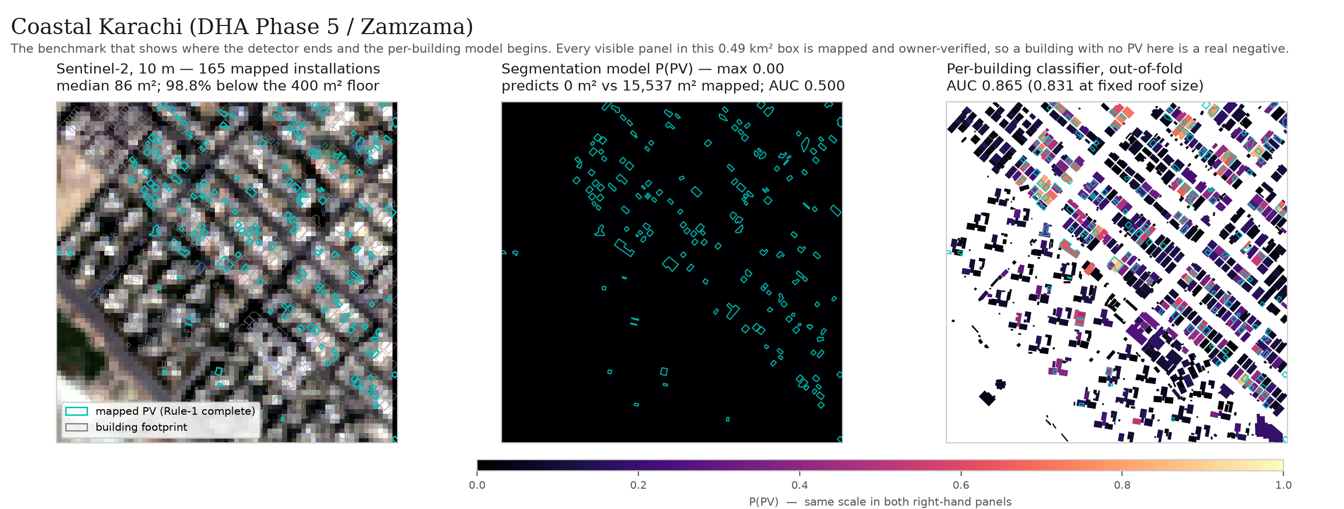
The coastal Karachi benchmark, the project's only Rule-1-complete quadrat. Same extent and same colour scale in the two right-hand panels. The segmentation model returns identically zero across the whole box; the per-building classifier, scored out of fold, separates the same roofs at 0.831 AUC with roof size held fixed. Regenerate with python scripts/plot_calib_quadrat.py.

That middle panel is the finding, not an illustration of it. It is the published detector on a box where 165 installations are mapped and owner-verified, and its output is not a faint signal but a uniform zero.

Leave-one-quadrat-out, 22,044 buildings and 2,376 carrying PV across nine quadrats (updated 2026-07-29 with the three owner-mapped boxes added that day: Mardan, Quetta, Sialkot). Adoption rises with house size, so footprint area alone already scores about 0.72; the within-size-band column removes size as a discriminator and measures what the imagery adds at fixed roof size, which is the honest headline.

held-out quadrat	base rate	AUC	AUC <500 m2	within size band	segmentation, within band	packing (m)
Karachi DHA 5 coastal (Rule-1)	0.185	0.883	0.886	0.846	0.500	16.8
Lahore DHA (residential)	0.301	0.876	0.876	0.761	0.496	7.2
Sialkot Old City	0.057	0.816	0.817	0.770	0.500	18.8
Mardan (Sheikh Maltoon Town)	0.138	0.743	0.742	0.661	0.500	11.2
Quetta City	0.030	0.852	0.856	0.842	0.501	44.0
Faisalabad PSIE	0.125	0.850	0.813	0.831	0.651	45.8
Multan Industrial	0.086	0.932	0.915	0.919	0.805	50.8
SITE Karachi	0.131	0.935	0.929	0.931	0.875	46.2
Sundar Industrial	0.098	0.874	0.840	0.863	0.762	52.1
median		0.874	0.856	0.842	0.501

The three new folds lower the median AUC slightly (0.879 -> 0.874) and the within-size median a touch more (0.845 -> 0.842) -- Mardan in particular is the weakest fold measured so far (0.743), the first non-industrial, non-Rule-1 quadrat in the set. Read that as the estimate becoming more honest with more evidence, not as the method degrading.

Packing distance: a cheap, measured proxy for stratum

packing (m) is roofclf.packing_density: the median distance from each sub-400 m² installation to its nearest neighbour of any size, in metres -- added 2026-07-29 and now computed automatically for every fold (folds.csv), not a one-off calculation. It splits the nine quadrats cleanly at ~20-40 m with no quadrat in between: five pack sub-400 m² arrays tighter than one Sentinel-2 pixel (7-19 m -- Lahore, Mardan, Karachi coastal, Sialkot), four sit at 44-52 m (Quetta, Faisalabad, Multan, SITE Karachi, Sundar).

That split is not incidental. Measured against the same nine quadrats' own numbers: packing distance correlates r=0.70 with exp_scale_anchor's fraction-head scale, r=0.82 with its segmentation scale, and r=0.78 with auc_within_size above. A single geometric measurement from the labels alone -- no imagery, no model -- predicts most of why quadrats disagree on exp_scale, rate_ratio, and skill. It is effectively a continuous, measurable version of the "4 industrial vs 5 residential" split this project already tracked by hand.

What packing distance is a proxy for

Those correlations hold, but they are mostly installation size wearing a spacing costume: control for median installation size and packing distance's relationship with segmentation skill collapses from 0.819 to -0.155. The one part that survives the control is its relationship with the fraction head's AUC (0.931 -> 0.809 partial), which is the genuine 10 m pixel-mixing effect. Full derivation, and the same treatment of base_rate, in Density and detection quality.

Two consequences, both acted on already:

• Held-out quadrat choice for the fraction-head retrain (below) should account for packing, not just be picked for convenience. Lahore, the densest quadrat (7.2 m), is also the single richest source of graded per-pixel training signal for the sub-400 m² regression target -- holding it out is a real trade-off (removing the best training example) made deliberately because it is also the most statistically powerful validation check (1,033 installations to test against, more than the other four dense quadrats combined).
• nn_median_m is now a standing column in evaluate()'s fold report, so any future fold's AUC/rate_ratio swing can be read against its packing regime at a glance, instead of needing a separate cross-reference. It is not (yet) used as a per-building model feature -- it is a quadrat-level property, not a building-level one, so it belongs in the reporting layer, not MODEL_FEATURES.

The two residential folds are the ones to read, and the coastal Karachi box is the strongest evidence in the project. It is the only quadrat asserted Rule-1 complete, so its PV-free buildings are trustworthy negatives rather than unmapped ones; its median installation is 86 m² and 98.8 percent of its installations sit below the detection floor. There, the segmentation model scores exactly 0.500, chance, and predicts zero PV area over the box's buildings. The per-building classifier reaches 0.831 at fixed roof size. Controlling for size costs the classifier only about 3 AUC points across folds, so this is the imagery separating a PV roof from a PV-free roof of the same size, not a house-size proxy.

A feature-block ablation sets the shipped configuration, rather than preference (also updated 2026-07-29, nine quadrats):

features	AUC	AUC, roofs <500 m2
footprint size only	0.715	0.668
footprint reflectance only	0.841	0.845
size + reflectance (default)	0.874	0.856
plus segmentation and fraction rasters	0.876	0.858

Size alone is a real but modest prior, so the skill is not just "big buildings have PV". With six quadrats, adding the existing model rasters as features cost accuracy on small roofs (0.882 -> 0.870); with nine, that reverses to a marginal gain (0.856 -> 0.858) -- small enough either way (<0.002) to read as noise rather than a real effect in both directions. The rasters stay off by default: the case for including them was never strong, and it is not stronger now.

Ranking transfers, absolute rates do not

rate_ratio in folds.csv spans 0.235 to 4.833 across nine quadrats (Mardan under-predicts 4.3x, Quetta over-predicts 4.8x). Trained pooled, the model predicts 0.137 for residential Lahore where the truth is 0.301. So the ordering generalises out of stratum but the level does not, and a per-stratum intercept is required before any adoption rate or capacity number is published. That needs more residential/non-industrial quadrats -- five of nine now cover that ground (Karachi coastal, Lahore, Sialkot, Mardan, Quetta), up from one, but the spread above shows the binding constraint has not gone away.

Density and detection quality: what actually correlates with what

This project has asserted a density-vs-detection-quality relationship in several places -- the packing-distance r values just above, and the rate_ratio spread in the warning box. Recomputed in one pass across every quadrat artifact on disk (scripts/quadrat_correlations.py -> results/quadrat_detection_correlations.csv, pixi run quadrat-correlations), the relationship is real but it is two different findings, and neither is "denser landscapes are harder in some intrinsic way." Both turn out to be artifacts with a specific fix, which is more useful than a correlation would be.

The script keeps two things apart on purpose, because conflating them is how "denser is worse" gets asserted: discrimination (can the instrument tell a PV pixel or building from a non-PV one within the quadrat -- the *_auc* columns, scale-free) and bias (does it predict the right amount -- scale, rate_ratio). A quadrat can rank perfectly and still be 3x high, so a correlation with one says nothing about the other.

Discrimination: it is installation size, not density

Every density measure correlates strongly with segmentation skill, and every one of those correlations disappears once installation size is held constant (n=9, Spearman, partial correlation controlling for median_install_m2):

relationship	Pearson r	Spearman rho	partial r given median size
median_install_m2 vs segmentation AUC	0.991	0.932	--
frac_sub400 vs segmentation AUC	-0.981	-0.932	-0.241
packing distance vs segmentation AUC	0.819	0.915	-0.155
installations per km² vs segmentation AUC	-0.603	-0.915	+0.201
frac_sub400 vs segmentation AUC within size band	-0.954	-0.932	+0.224
median_install_m2 vs fraction-head pixel AUC (n=12)	0.889	0.888	--

Median installation size is the single best predictor of whether the segmentation raster works at all, at r=0.991 -- which is not a subtle empirical finding but the detection floor doing exactly what it says: the model is trained with everything below chips.MIN_PV_AREA burned as ignore, so a quadrat whose installations are mostly small gets chance-level output. Dense quadrats score badly because dense quadrats are dense in small installations, not because density itself hurts. Controlling for size, packing distance's relationship with segmentation skill goes to -0.155 and installations-per-km² actually flips sign.

One relationship survives the control, and it is the mechanistically expected one: packing distance vs the fraction head's per-building AUC, 0.931 unconditionally and 0.809 partial. That is the one place a spacing effect should appear independent of array size -- the fraction head predicts per-pixel coverage, and what spacing controls at 10 m GSD is how much of a pixel a neighbouring array contributes. roofclf.packing_density's median 15-17 m in the densest quadrats is at or below one pixel, so neighbours mix into each other regardless of how big any one of them is.

So packing_density remains a useful cheap stratum proxy -- but for installation size regime first and spectral mixing second, not for density as such. That is a correction to how the r=0.70-0.82 figures above were framed, not a retraction of them.

Bias: the base-rate correlation is mechanical

base_rate is the strongest correlate of bias in the whole table, at rho=-0.950 (p=0.0001, n=9), and unlike the discrimination results it survives controlling for installation size (partial r=-0.765). Higher true adoption, more under-prediction. It is also almost entirely an arithmetic consequence of a missing intercept:

• The model's predicted rate is essentially unrelated to the truth: pred_rate vs base_rate is r=-0.167 (p=0.67), rho=-0.417 (p=0.27).
• pred_rate is nearly flat -- mean 0.137, sd 0.043, CV 0.31 -- while base_rate spans 3.0% to 30.1%, CV 0.62. The classifier predicts roughly one number everywhere.
• So rate_ratio = pred_rate / base_rate reduces to constant / base_rate. Substituting the mean predicted rate for pred_rate reproduces the observed rate_ratio at r=0.969, rho=0.950, median relative error 8.9%.
• A log-log fit gives slope -1.133, where exactly -1.0 is the purely mechanical hyperbola.

The "crossing point" this project has described at ~12% base rate is therefore not a property of Pakistani settlement: rate_ratio = 1 at base_rate 12.3% simply because that is where the flat predicted rate happens to meet the truth, and it sits right next to the training quadrats' own mean base rate (12.8%). Recalibrating on a different set of quadrats would move the crossing point to that set's mean, without the model having learned anything new.

Read that as confirmation of the fix already on record rather than a new obstacle: a per-stratum intercept is the thing missing, and rate_ratio's 0.235-4.833 spread is what a missing intercept looks like when you divide by a base rate that varies 10x. Mardan is the one quadrat the mechanical account does not fit (pred_rate 0.032 against a flat ~0.137), which is consistent with it being the weakest fold on independent grounds.

One bias relationship is not mechanical and is worth keeping: frac_sub400 vs the fraction head's predicted/true area, r=-0.945 / rho=-0.841 (n=12) and -0.691 partial. The more of a quadrat's PV sits below the detection floor, the more area the instrument misses -- the sub-400 m² blindness measured directly, and the reason the sub-400 m² instruments exist at all.

How much to trust these numbers

n is 7-13 per pair and the script tests 72 pairs, so no single p-value here is evidence on its own. What carries the weight is that the two headline results are each pre-registered by an earlier claim in this document (packing distance predicts skill; rate_ratio varies with base rate) and each has a mechanism that predicts the sign and rough magnitude in advance -- a detection floor at 400 m², and a classifier with one pooled intercept. The partial correlations are computed on a single control with n=9, so treat them as directional, not precise. Re-run the script when a quadrat is added; that is the check that matters more than any p-value in it.

National deployment: a scaling success, with one clean calibration lesson

roofclf.score_buildings_national takes the pooled fit above and scores every VIDA building in the country -- 81.76 million buildings across all 4,473 composite cells, previously untested at this scale. Two things made it tractable rather than a multi-day job: the shipped feature set never needed the segmentation/fraction probability rasters (ablation-excluded, see the table above), so scoring needs only composites + VIDA buildings, both already proven at national scale by density.py; and routing through local_source.composite_index's existing lru_cache (previously unused by anything) avoids rebuilding the ~4,474-tile composite index once per cell. The deployment threshold is chosen the same way as the SPPI work (sppi._precision_threshold): most conservative cut clearing a target precision on pooled leave-one-quadrat-out scores, not Youden's J, because a capacity-contributing detector needs precision as the primary criterion.

That threshold is also where the "ranking transfers, absolute rates do not" warning above stopped being abstract. Quetta -- the lowest-base-rate quadrat by a wide margin (3.0%, next-lowest is 5.7%) and the one place SPPI's own building-scoped detector collapsed to 10.5% precision -- was distorting the pooled threshold: holding a 0.50 precision target across all nine quadrats forced the cut up to 0.4555, which caught only 25% of true positives at that precision. Re-fitting on the other eight quadrats (Quetta excluded, data/roofclf_with_quetta_20260730/ kept for comparison) relaxed the threshold to 0.3064 and recall at the same 0.50 precision target rose to 39.6% -- a real, measured gain from removing one quadrat whose extreme base rate was pulling the whole pooled cut in the wrong direction, not from more data or a better model.

What this experiment does and does not license. It is a genuine win on the question roofclf was built to answer -- given a fixed precision bar, how many true installations does the flagged set catch -- and it is the clearest illustration yet of why a single pooled cut is fragile: one outlier stratum, not nine ordinary ones, was setting the whole country's operating point. It does not mean roofclf's national output is ready to contribute a capacity number. Converting 872,730 incrementally flagged buildings (no segmentation candidate within 30 m) into MWp at a flat precision weight was tried and produced 18,063 MWp -- 3.5 to 8x the country's entire existing recall-corrected total -- because a flat precision measured on nine base-rate-skewed quadrats does not survive being applied to 81.76 million mostly-rural buildings at a different true prevalence, the same failure this section's warning already names. See the full writeup for the diagnosis. roofclf's national scores stand today as a per-building ranking/lead-generation signal, not a capacity input.

SPPI cross-validation: real but uneven, and only as a second opinion

SPPI (He et al. 2026, src/earthpv/sppi.py) is a zero-training spectral index scored directly on roofclf's own held-out ground truth (data/roofclf/buildings.geoparquet) -- the same 8 quadrats, same labels, apples to apples:

signal	median AUC	within size band
SPPI (zero training)	0.823	0.828
roofclf (17 features, fitted)	0.874	0.842

roofclf wins, but not by a wide margin given SPPI needs no training at all. Adding SPPI as a roofclf input feature does nothing -- 0.8736 to 0.8734 AUC, the same within-noise result the seg/frac raster features got when tried the same way -- because roofclf's fitted linear weights already span the bands SPPI computes a fixed nonlinear combination of. That could read as "SPPI is redundant, stop here." It is not: a second, independent check does something a single linear model over the same bands cannot, tested 2026-07-30 as a live question ("could both methods agreeing produce a conservative sub-400 m² estimate?") rather than assumed.

Restricting to sub-400 m² buildings (8 quadrats, Mardan excluded as its own already-diagnosed bad fold) and requiring roofclf >= 0.3064 and SPPI above a matched-recall threshold:

	precision	recall	n flagged
roofclf alone	0.496	0.462	1,144
AND-gate (both agree)	0.540	0.445	1,009
roofclf alone, at the same recall (0.445)	0.498	--	--

Agreement buys roughly +4 points of precision over roofclf alone at matched recall -- a real, measured gain, not just a stricter cutoff on one model wearing a different hat. The mechanism: SPPI is a fixed nonlinear combination of bands, roofclf a linear model over similar bands -- a linear model cannot fully reconstruct a nonlinear AND from one added covariate, so the two decision boundaries stay genuinely complementary even though SPPI carries no rank information roofclf doesn't already have on its own.

The gain is real but concentrated, not uniform -- read per quadrat, as always:

quadrat	roofclf precision	AND-gate precision	delta
Multan	0.256	0.363	+10.7pp
Sialkot	0.321	0.376	+5.5pp
Sundar	0.253	0.304	+5.1pp
SITE Karachi	0.567	0.581	+1.4pp
Lahore	0.791	0.795	~flat
Faisalabad	0.359	0.352	-0.7pp
Karachi coastal	0.644	0.635	-0.9pp

The gain concentrates almost entirely in Multan/Sialkot/Sundar -- exactly the three low-base-rate quadrats the density-stratified precision work above had to exclude from calibration because roofclf overestimates 2x+ there. That is a coherent story, not a coincidence: SPPI agreement specifically catches roofclf's overconfidence in the regime already known to be miscalibrated, rather than helping everywhere.

Tested nationally, 2026-07-30, on the domain-restricted population -- and it does not help there, confirming the table above rather than adding to it. score_buildings_national now saves sppi alongside p_roofclf (zero extra cost, same bands already read; re-run once to backfill it, data/roofclf_national_with_sppi/pakistan/prob/). Applying the AND-gate to the same 93 domain-restricted cells the sub-400 capacity figure below uses (i.e. exactly the Faisalabad/Karachi-coastal/SITE-Karachi-like regime, not Multan/Sialkot/Sundar): precision on those three calibration quadrats themselves is flat (0.5501 roofclf-alone vs 0.5499 AND-gate) while the AND-gate cuts the flagged population by 31% (496,122 to 343,032 buildings) and the resulting capacity figure by 29% (6,628 to 4,690 MWp) for no precision gain. This is the mechanistic prediction of the per-quadrat table above, confirmed rather than contradicted: SPPI's benefit lives specifically in the low-density quadrats the domain restriction already excludes, so stacking the AND-gate on top of an already-restricted, already-well-calibrated population only removes recall for free. Not adopted for the domain-restricted figure. SPPI remains valuable as a check in the regime it actually helps (a future, separate low-density correction, not yet designed), not as a blanket addition to every roofclf deployment.

Regime-B correction and a national-proxy test (2026-07-31)

Two follow-up questions, asked directly: does the Multan/Sialkot/Sundar-specific gain reproduce under a pooled (not per-quadrat) re-test, and can a per-cell signal tell us where that regime applies nationally so its correction could actually be deployed?

Reproduced, pooled, at matched recall. sppi.and_gate_regime_precision pools TP/FP/FN across Multan, Sialkot and Sundar (sub-400 m² buildings, 9-quadrat table) rather than reading off per-quadrat deltas one at a time:

	precision	recall
roofclf alone (0.3064 threshold)	0.309	0.424
roofclf alone, at the AND-gate's own recall	0.462	0.153
AND-gate	0.578	0.153

A +11.7 point pooled gain at matched recall, a bit larger than the mean of the three individual per-quadrat deltas (+10.7/+5.5/+5.1pp) reported above -- the effect survives pooling, it is not an artefact of averaging three small samples. The cost is the same one already on record: only 15% of true installations in this regime survive the AND-gate. This is now reusable code (sppi.and_gate_regime_precision), not a one-off script result.

A related instability worth naming. Which quadrats even count as "Multan/Sialkot/ Sundar-like" (rate_ratio outside [0.5, 2.0]) depends on which fold table you read, because rate_ratio is itself a leave-one-quadrat-out statistic that shifts as the training pool changes. Sundar measures 1.68 (7-quadrat table), 2.11 (8-quadrat, Mardan added), then 1.71 (9-quadrat, Quetta added) -- straddling the 2.0 boundary across runs. The domain-restricted capacity figure (6,628 MWp) used the 8-quadrat table's 3-quadrat split (Faisalabad, Karachi coastal, SITE Karachi); re-running select_calibrated_quadrats against the current 9-quadrat table gives 4 (Sundar now included). This does not change the 6,628 MWp figure retroactively -- that number is pinned to the fold table it was computed from -- but it means the Good/Regime-B split is a measurement with its own sampling noise near the boundary, not a fixed partition of Pakistan's geography.

Per-cell SPPI agreement rate as a national stratification proxy: tested, and it does not work. The real, reproduced gain above is useless for national deployment without a way to tell which national cells are Multan/Sialkot/Sundar-like versus Faisalabad/Karachi-coastal/SITE-Karachi-like -- exactly the proxy problem this project has already failed to solve twice (existing candidate density anti-correlates with true small-PV rate; roofclf's own raw predicted rate does not separate the regimes either). A per-cell signal needs no ground truth to compute nationally, so a candidate worth testing before assuming it does not exist: does the fraction of roofclf-flagged buildings that SPPI also confirms (sppi.agreement_rate_by_quadrat) track rate_ratio?

quadrat	confirmation rate	rate_ratio
Mardan	0.000	0.235
Lahore	0.050	0.454
Karachi coastal	0.098	0.682
SITE Karachi	0.440	1.146
Faisalabad	0.675	1.328
Sundar	0.319	1.710
Multan	0.327	2.068
Sialkot	0.117	2.304
Quetta	0.506	4.833

Correlation among the 7 quadrats with an ordinary failure mode (excluding Mardan and Quetta, each already separately diagnosed as a distinct problem, not a density-regime one) is weak: Pearson r = 0.19, Spearman rho = 0.36. It only looks strong (r = 0.50, rho = 0.63) with Mardan and Quetta folded back in -- almost certainly driven by those two known outliers rather than a real relationship, since the sign is not even consistent among the core 7: Karachi coastal (well-calibrated, rate_ratio 0.68) shows a lower confirmation rate than Sundar (over-predicting, rate_ratio 1.71), the opposite of what the hypothesis predicts. Negative result, kept as code (sppi.agreement_rate_by_quadrat) rather than deleted, in the same spirit as roofclf_capacity.py: this project has now failed to find a national stratification proxy three times (candidate density, roofclf's own rate, SPPI agreement rate), which is itself useful to know before trying a fourth. The Regime-B correction above therefore stays exactly where it started: a real, reproducible effect with no known way to say where it applies outside the quadrats it was measured on.

Sub-400 m² experimental capacity: density-stratified, deliberately separate

src/earthpv/sub400_capacity.py (2026-07-30) is the outcome of trying to fold both sub-400 m² instruments -- the fraction head and roof-classifier's national scores -- into one capacity number. It is not part of the published atlas above, on purpose: promoting the fraction head into density.py itself broke check-density (previous section), and the module's own docstring is written as a running record of what was tried and rejected, not just what worked, in the same spirit as roofclf_capacity.py.

Precision correction alone does not fix national deployment. roofclf's per-quadrat precision at the deployment threshold (0.3064) is not flat -- it ranges 0.30 to 0.81 across the 8 (no-Quetta) calibration quadrats -- and the relationship to true PV density (base_rate) is a crossing point, not a slope: quadrats below about 12% base rate over-predict by 2x or more, the one quadrat well above it (Lahore, 30%) under-predicts instead, and Mardan is a separate, already-diagnosed bad fold unrelated to density. Restricting to the three quadrats whose rate_ratio sits within 2x of 1 either way (Faisalabad, Karachi coastal, SITE Karachi -- 12.5-18.5% base rate) lifts pooled precision from the flat LOQO 0.499 to 0.5495. Applied to the same national population the rejected flat-precision attempt used, this makes the number worse, not better -- 37,197 to 40,879 MWp -- because 0.5495 is still just barely above 0.5. The volume of buildings being priced, not the weight applied to them, was always the problem.

What actually moves the number is restricting the population. Combining three corrections -- the pre-existing building-density domain restriction (only the 93 of 4,473 national cells whose settlement density falls in the calibration quadrats' 737-4,750 bldg/km² range), a contamination filter (buildings whose own footprint is already >= 400 m² are dropped from "incremental" -- they were never sub-floor, they just sit outside new_lead_mask's 30 m matching radius of an existing candidate; 13.4% of the domain-restricted incremental buildings, 49% of its area), and the density-regime precision above -- gives:

	value
Domain cells	93 / 4,473 (2.1%)
Buildings in domain	15.6M / 81.8M (19.1%)
Incremental buildings (post-contamination-filter)	418,076
Incremental sub-400 m² roof area	67.0 million m²
Sub-400 m² capacity (domain-restricted)	6,628 MWp

That is, for the first time, the same order of magnitude as the country's entire existing segmentation-based total (5,078 MWp) rather than 3.5-8x it. It is still not a national number: 6,628 MWp describes only those 93 cells. Rescaling it by the domain's 2.1%/19.1% share to infer a country total (~315 GWp) is exactly the base-rate-transfer failure this module exists to avoid, and domain_restricted_capacity's returned summary states the scope explicitly so a caller cannot lose that caveat downstream.

Where those 93 cells are (the only areas this figure actually describes): Karachi, Lahore and Peshawar (7-8 cells each), Mardan and Faisalabad (6), Islamabad and Sialkot (5), Multan, Charsadda, Sheikhpura and Gujranwala (3), Rawalpindi and Quetta (2), plus a long tail of single-cell districts. Building density (not PV density) is the only national proxy that survived testing as a way to identify candidate areas -- existing segmentation-detected candidate density was tried and rejected: it anti-correlates with true small-PV base rate (Karachi coastal and Lahore, the two quadrats with the highest true small-PV adoption, both show near-zero existing large-PV candidate density, because large-industrial and small-residential PV are different populations). roofclf's own raw predicted rate per cell was also tried and rejected: it does not separate calibrated from miscalibrated quadrats either (Multan and Sundar's predicted rate sits inside the "well-calibrated" band despite being 2x+ miscalibrated in truth). So "where might medium/high sub-400 m² PV density exist beyond the 8 mapped quadrats" is answered here only as "these are the largest, densest cities, which is where 6 of the 8 existing quadrats already are" -- a reason to prioritize new calibration quadrats in Karachi's other residential districts, Rawalpindi, Peshawar and Islamabad, not a validated prediction of where capacity sits.

A sub-400 m² capacity bracket, plus non-imagery anchors (2026-07-31)

Everything above answers "how much capacity does a detector find." This section asks a different question: given that both instruments are known to need a per-stratum correction that does not exist yet, what is a defensible range, and does anything independent of imagery corroborate it? Two frames, kept explicitly separate -- mixing them is exactly the base-rate-transfer mistake this page documents repeatedly.

The Low/Central/High bracket members below are resolved per 0.1° cell (not just as national totals) in an interactive atlas, switchable between four views: results/pakistan_pv_sub400_bracket_atlas.html (atlas.build_sub400_bracket_atlas, earthpv atlas --sub400-low-cells ... --sub400- central-cells ... --sub400-high-cells ...). Large PV (>= 400 m², recall-corrected) is always shown too, per a follow-up request (2026-07-31): for Low and Central it is added into the reported total using the ROOFTOP-scope figure only (large PV nationwide plus small PV inside the checked cells, the same "large everywhere, small where checked" combination build_combined_atlas already ships for its single roofclf-alone case, now extended to both Low and Central); for High it is shown for scale only and not added in, since High is an explicit, uncalibrated ceiling and folding it together with the project's main validated number would blur that distinction. The atlas still reports each view's small-PV-only component alongside the combined figure, so nothing here is hidden, only added to.

A fourth view, All-PV, answers a deliberately different, wider question: Central's small-PV component (roofclf alone, the 93-cell domain) plus large PV across EVERY placement, ground-mount farms included (est_mwp_rc, not est_mwp_rc_roof) -- 11,706 MWp nationally (6,628 small-PV + 5,078 large all-placement). This is kept separate from Central rather than used as Central's own headline number, for two reasons requested and confirmed the same day: ground-mount is a different physical asset class than "how much PV small buildings carry," with its own site-area conversion constant, and it is this pipeline's most bug-prone component (the ground-mount-to-rooftop ratio check in plausibility.py exists specifically because of it) -- so folding it in does not raise certainty, it adds a different kind of risk under a number that would otherwise read as a rooftop total.

Frame A -- domain-restricted (93 of 4,473 cells, 19.1% of buildings, NOT a national figure). The existing roofclf-alone figure above (6,628 MWp) gets a new companion, requiring roofclf and SPPI to agree instead of roofclf alone -- sub400_capacity.domain_restricted_and_gate_capacity (new this session; the AND-gate was previously measured only in an unsaved ad hoc script, reported in prose two sections up as 4,690 MWp). Re-measured with a properly pooled (not in-sample-ad-hoc) SPPI threshold fit on the same three calibration quadrats:

	roofclf alone	AND-gate (roofclf & SPPI)
Precision (on the 3 calibration quadrats)	0.5495	0.6166
Recall (same quadrats)	0.7226	0.5839
Flagged buildings (93-cell domain)	496,122	187,740
Sub-400 m² capacity (this domain only)	6,628 MWp	2,651 MWp

Unlike the earlier prose result (flat precision, recall traded away for nothing), the properly pooled threshold shows the AND-gate buys a real +6.7 point precision gain, not just a stricter cut at the same precision -- the earlier 4,690 MWp figure is superseded by this one; it was never saved as reusable code and is not exactly reproducible. Both remain scoped to the same 93 cells -- do not rescale either to a country total, for the reason stated repeatedly above.

Frame B -- unrestricted national, explicitly uncalibrated. Refreshing the flat-LOQO- precision fold-in (roofclf_capacity.incremental_capacity) at the current deployment threshold (0.3064, post-Quetta-exclusion) against the full national scoring output reproduces 37,196.6 MWp -- matching the 37,197 MWp already on record in sub400_capacity.py's docstring, confirming the number is stable under a fresh read of the current artifacts. This supersedes the older 18,063 MWp figure, which used the prior 9-quadrat 0.4555 threshold (since relaxed) and is not directly comparable. This is offered as a ceiling only, per the go-ahead to publish an upper bound that "does not need to be fully calibrated or validated" -- the precision weight is known not to survive the prevalence shift from 9 urban/industrial quadrats to 81.76M mostly rural buildings (see above), so treat it as an outer bound on plausibility, not an estimate.

External, non-imagery anchors. Two independent administrative/trade data points, neither derived from this pipeline at all:

• NEPRA net-metering register (Pakistan's regulator, the closest available analogue to Germany's MaStR): 5.3 GW registered nationally by April 2025 across 283,000 consumers, projected to reach 6.3 GW by the end of FY2024-25 (pv magazine, pv magazine). Average registered size is 18.7 kWp/consumer -- well under the model's 72 kWp (400 m²) floor, so this register is itself dominated by exactly the sub-400 m² population this section is about. It is a floor, not a total: it only counts customers who completed DISCO net-metering paperwork, and Pakistan's solar boom is widely reported as running well ahead of formal registration (self-consumption and off-grid/battery installs never appear here at all). Frame B's ceiling (37.2 GWp) sitting roughly 6-7x above this floor is consistent with that gap, not contradicted by it.
• Cumulative panel imports: Chinese customs data puts Pakistan's 2024 solar panel imports at 16.91 GW, up from 7.47 GW in 2023 (+127%), with trade press citing roughly 50 GW cumulative by August 2025 (pv magazine, Renewables First/Taiyang News). This is a much looser anchor -- it is import volume, not installed rooftop capacity, and conflates utility-scale procurement, warehoused stock, and re-exports with rooftop installs of every size. It is included only as an order-of-magnitude sanity check: the gap between it and the NEPRA floor is the same "unregistered solar" phenomenon Pakistani energy press already documents, and it is large enough that nothing in this bracket is anywhere near implausible on these grounds.
• MaStR-shape-implied ceiling. Applying Germany's legally complete size split (72.6% of rooftop capacity in units <=100 kWp, ~<=555 m² of module; see "How the estimate got here" below) to this project's own current published >= 400 m² rooftop total -- 2,229.9 MWp, recall-corrected, summed directly from data/predictions/pakistan/density/grid.geoparquet (the per-cell source of truth; an earlier draft of this section misread regions.csv, which stores BOTH province- and district-level rows summing to the same national total each, and summed across both, doubling it to 4,457 -- corrected 2026-07-31) -- implies a sub-400 m² total of order (0.726/0.274 =) 2.65 x 2,230 approx 5,900 MWp, if Pakistan's roof-size distribution resembled Germany's. Two named caveats: the 400 m² vs. ~555 m² cutoff mismatch, and no evidence yet that a mostly-rural, much poorer country's roof-size distribution resembles Germany's at all. It lands close to Frame A's central figure, which is the most it should be read as saying.

bracket member	value	scope	mechanism
Frame A, AND-gate (low)	2,651 MWp	93 cells only	roofclf & SPPI agree, density-restricted
Frame A, roofclf-alone (central)	6,628 MWp	93 cells only	roofclf alone, density-restricted
MaStR-shape-implied	~5,900 MWp	national (implied)	Germany size-distribution transfer
NEPRA net-metering	5,300-6,300 MWp	national (registered only)	admin record, non-imagery
Frame B (high)	37,197 MWp	national, unrestricted	flat LOQO precision, explicitly uncalibrated

Read this table by column, not by sorting the value column. The two Frame A rows and the Frame B row describe different populations (2.1% of cells vs. 100%) and must not be combined or rescaled into each other. NEPRA and MaStR are the only two rows that are genuinely national and independent of this pipeline. The MaStR-implied figure lands close to Frame A's own central estimate despite sharing no inputs with it -- two disjoint methods agreeing that closely is the strongest corroboration in this table. Frame B's explicitly uncalibrated ceiling sits a further 6x above both, comfortably above the NEPRA floor either way; that gap is consistent with "not implausible" for an explicit ceiling, not evidence that 37,197 MWp is itself a good estimate.

Total capacity as a pipeline input

Every number above is this project's own estimate of the total. earthpv redistribute-capacity (capacity_redistribution.py) answers a different question: given a total from an independent, possibly more-trusted source (for example Pakistan's NEPRA net-metering register), how should that total be spread across cells, regions or buildings, using this project's own measured relative shape rather than its absolute number: share = row's est_mwp_* value / (national or per-region) sum, distributed = share x external_total. It reads density/'s finished outputs and writes its own sibling file, never touching grid.geoparquet/regions.geoparquet in place.

Two caveats worth stating plainly: an external total necessarily includes small (< 400 m²) PV, so distributing it by the ≥ 400 m² shape this project can actually validate assumes small-PV's spatial distribution tracks large-PV's, which is not established; and the transform is point-estimate only, since est_mwp_rc's posterior credible interval is not currently propagated through it.

earthpv redistribute-capacity --aoi pakistan --total-capacity 5800 --scope national

--scope region (one total per region, each spread by that region's own local shape) is built and wired the same way, but has no real companion data yet -- no provincial NEPRA breakdown exists in this project's sources today, only the national scalar above.

Rooftop potential and saturation

Everything above answers "how much PV is already there." earthpv atlas --potential-buildings <path> (atlas.py::build_potential_atlas, potential.py::large_roof_buildings) answers a different, forward-looking question: where are large, currently-uncovered roofs that would make good candidates for future rooftop solar, and where is existing adoption already dense vs. sparse. It is a two-tab atlas, not a new capacity estimator, kept deliberately separate from every number above.

Potential. Every VIDA building nationally with roof_area_m2 >= 200 is pulled from roofclf.score_buildings_national's existing per-cell output, reusing only that table's building-footprint geometry, never its PV-presence scores -- this instrument only measures building footprint size, so none of roofclf's calibration/precision caveats apply here. From each cell's total large-roof area, the segmentation model's own probability-weighted expected PV area is subtracted to get an uncovered large-roof area, which converts to peak capacity at the usual 0.18 kWp/m² module constant and then to annual energy via a PVGIS-modelled specific yield. 200 m², not the 400 m² detection floor, is the cutoff because it reaches further into the realistic rooftop-opportunity space (roughly where Germany's MaStR register shows most rooftop capacity actually sits) rather than merely restating the population already above the detection floor -- with the caveat that the segmentation model has no discriminating signal at all in the 200-400 m² band, so that band's "potential" reads as almost entirely uncovered regardless of whether PV is actually there.

Saturation. This tab adds no new computation: pv_ratio_det/pv_ratio_exp (PV area over roof area) are already computed per cell and region and land unconditionally on grid.geoparquet/regions.geoparquet. The tab exists purely to give that existing ratio its own choropleth view.

Leads. scripts/build_potential_leads.py (pixi run potential-leads) ranks individual large, uncovered roofs by roof_area_m2 * kwh_per_kwp_yr at the building's own cell, drops anything within 30 m of an existing detected candidate or hand-mapped OSM solar feature, and caps at 6 per 0.1 deg cell, for a human to spot-check the highest-opportunity roofs before treating any of this as validated.

The plausibility gate

The leads product has a human on every candidate. The capacity atlas has nobody, so a false-positive mode that survives the precision weighting reaches the published number silently: a province total simply comes out too large, and nothing in the pipeline objects. earthpv check-density is that objection, and it runs between density and publishing. It exits non-zero on a failure and 2 if the stage has not run, so it can gate a pipeline; the docs CI cannot run it, because the density outputs it reads are gitignored and live next to the rasters.

Two independent per-region checks, both computed from layers the stage already wrote:

Ground-mount against rooftop. Detections off a building are the dominant false-positive mode, and unlike a rooftop detection nothing constrains them to a plausible host. A region whose ground-mount estimate dwarfs its rooftop estimate is claiming utility-scale solar that would be independently documented if it existed. Suspect above three times, failing above five, with a 50 MWp floor so a tiny region's ratio is not noise.

Single-cell concentration. One 0.1 degree cell holding more than a quarter of a region's capacity means that region's total is one object, not a population, and no amount of per-bin calibration turns it into a statistic.

Current published state: 3 flagged regions, checked and published anyway

The published run fails the single-cell-concentration check for Khyber Pakhtunkhwa, Balochistan and Islamabad Capital Territory. All three flagged cells are the calibration quadrats' own cities (Peshawar, Quetta, Islamabad), which naturally dominate otherwise sparse regions once an earlier ground-mount overstatement (fixed by splitting rooftop and ground-mount calibration by placement) stopped masking that concentration. Gilgit-Baltistan is separately exempted from the ratio check via RATIO_CHECK_EXEMPT_REGIONS, because its real rooftop base rate is near zero and the ratio is structurally uninformative there. Published anyway, per this project's precedent for a checked-genuine plausibility failure. See Open questions.

Running it

# once, and again whenever new validation evidence lands
pixi run earthpv calibrate-candidates --aoi pakistan

pixi run earthpv density --aoi pakistan --districts
pixi run earthpv check-density --aoi pakistan  # gate the numbers before publishing them
pixi run earthpv atlas --aoi pakistan          # standalone atlas regeneration

Changing the expected-area instrument or --exp-scale only reaches the per-building and *_roof columns on a --force re-run, since those live in the cached cell partials. For the sub-400 m² instruments (roof-classifier, roofclf-score-national, sub400-capacity, ge400-roof-capacity), see The rooftop classifier and the capacity map's reproduction steps.

This system reached its current shape through several rounds of measurement against Germany's MaStR register and an independent Pakistani distributed-solar study, most notably the recall correction, the mounting-split conversion, and the plausibility gate itself, each added after a method review found the previous step alone was not enough. The full account of what was tried, what it cost, and what did not work (a fraction- regression head, a Low/Central/High bracket atlas, two-endmember spectral unmixing among them) is in Experiments; concrete open items are in Open questions.